@misc{grf,
  title        = {grf},
  author       = {Athey and Tibshirani and Wager},
  howpublished = {\url{https://grf-labs.github.io/grf/}},
  note         = {Software / documentation}
}A minimal first-contact recipe: regression forest, quantile forest, and a causal forest on the same data.
Input · what goes in
2,000 obs, 10 covariates X, a binary treatment W, continuous outcome Y.
Show data format & exampleHide example
Format — one row per unit. A covariate matrix X (numeric), a binary treatment W ∈ {0,1}, and an outcome Y.
  X1     X2    X3    W    Y
 0.42  -1.1   0     1   3.10
-0.07   0.6   1     0   1.85
 1.20   0.3   0     1   4.02
Pipeline · the recipe ⑂ has parallel branches
↑ Click any step in the diagram to read its logic, code, assumptions & discussion.
Assemble X, W, Y; check overlap
Data preparation — shapes the raw inputs into what the estimator expects.
One row per unit; numeric design matrix X, treatment W, outcome Y. Eyeball propensity overlap.
- No comments on this step yet — be the first.
Log in to comment on this step.
[GRF] Regression forest
The core estimate — where the causal quantity itself is computed.
Fit E[Y|X]; read off OOB predictions and variable_importance().
Regression forest — Honest non-parametric regression for E[Y|X], with out-of-bag predictions and pointwise CIs.
rf <- regression_forest(X, Y)
Y.hat <- predict(rf)$predictions
- No comments on this step yet — be the first.
Log in to comment on this step.
[GRF] Quantile forest
The core estimate — where the causal quantity itself is computed.
Fit conditional quantiles to see distributional, not just mean, structure.
Quantile forest — Conditional quantile estimation — the full predictive distribution, not just the mean.
qf <- quantile_forest(X, Y, quantiles = c(.1, .5, .9))
predict(qf, X.test)
- No comments on this step yet — be the first.
Log in to comment on this step.
[GRF] Causal forest
The core estimate — where the causal quantity itself is computed.
Fit CATEs with the same call shape; predict with estimate.variance = TRUE.
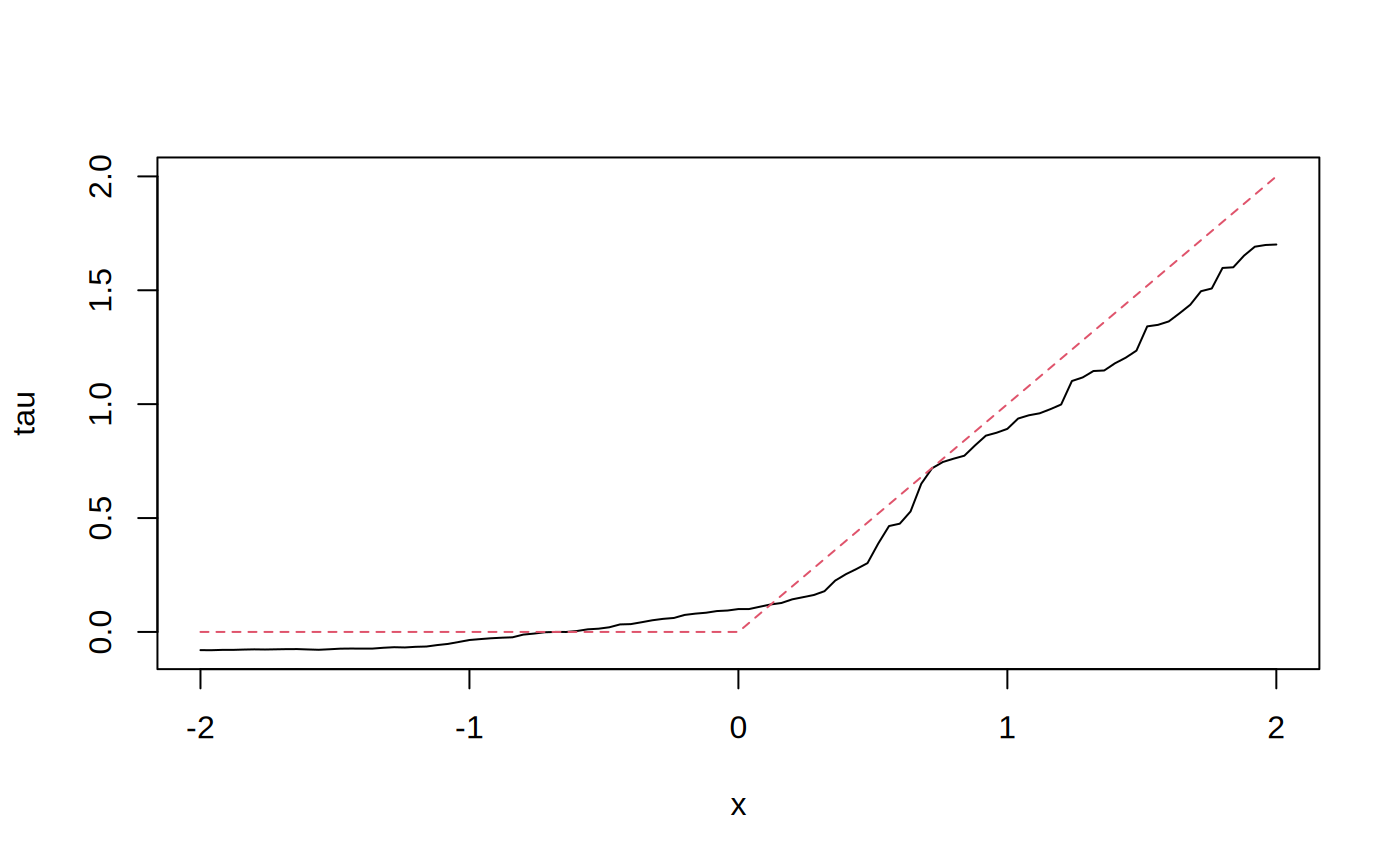
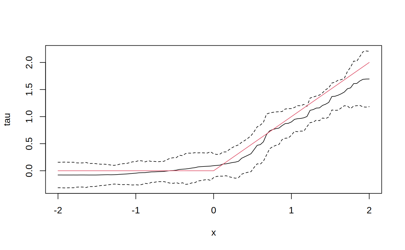
Causal forest — Honest random forest for heterogeneous treatment effects — CATE for a binary treatment via GRF moment conditions.
cf <- causal_forest(X, Y, W) # Y.hat, W.hat cross-fit
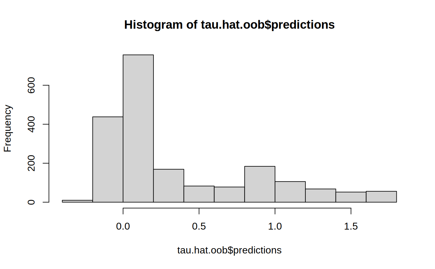
tau.hat <- predict(cf)$predictions # OOB CATEs
- No comments on this step yet — be the first.
Log in to comment on this step.
OOB predictions & variable importance
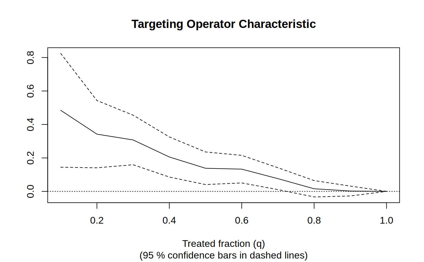
Reporting — turn the numbers into a figure or table a reader can act on.
Compare the three forests; show importance and a CATE histogram.
- No comments on this step yet — be the first.
Log in to comment on this step.
Output · what you get 4 figures
Figures reproduced from grf — Athey, Tibshirani & Wager — unofficial community showcase; all credit to the original authors.
The GRF 'introduction' vignette, distilled to a teaching recipe. Shows the shared API across forest types and where OOB predictions and variable importance come from. Unofficial summary.
Discussion (2)
Log in to join the discussion.
Perfect first-contact recipe. Showing the identical call shape across regression/quantile/causal forests is the fastest way to 'get' the package.
Would hand this to any new grad student. Clean.