Heterogeneous treatment effects with a causal forest (GRF recipe)
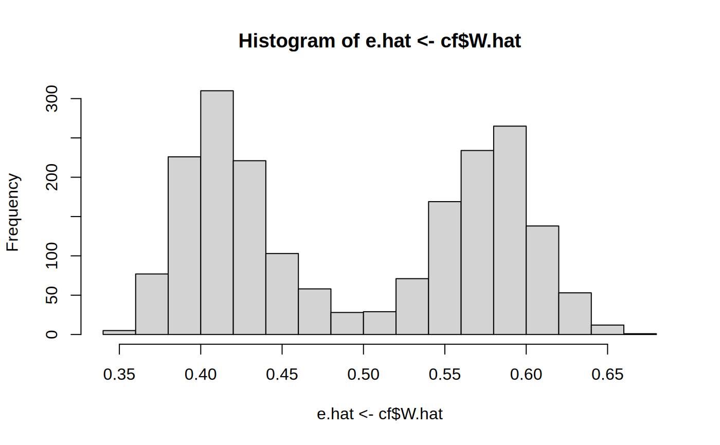
The full GRF HTE playbook: cross-fit nuisances → causal forest → calibration → AIPW ATE → BLP → RATE → policy.
The full GRF HTE playbook: cross-fit nuisances → causal forest → calibration → AIPW ATE → BLP → RATE → policy.
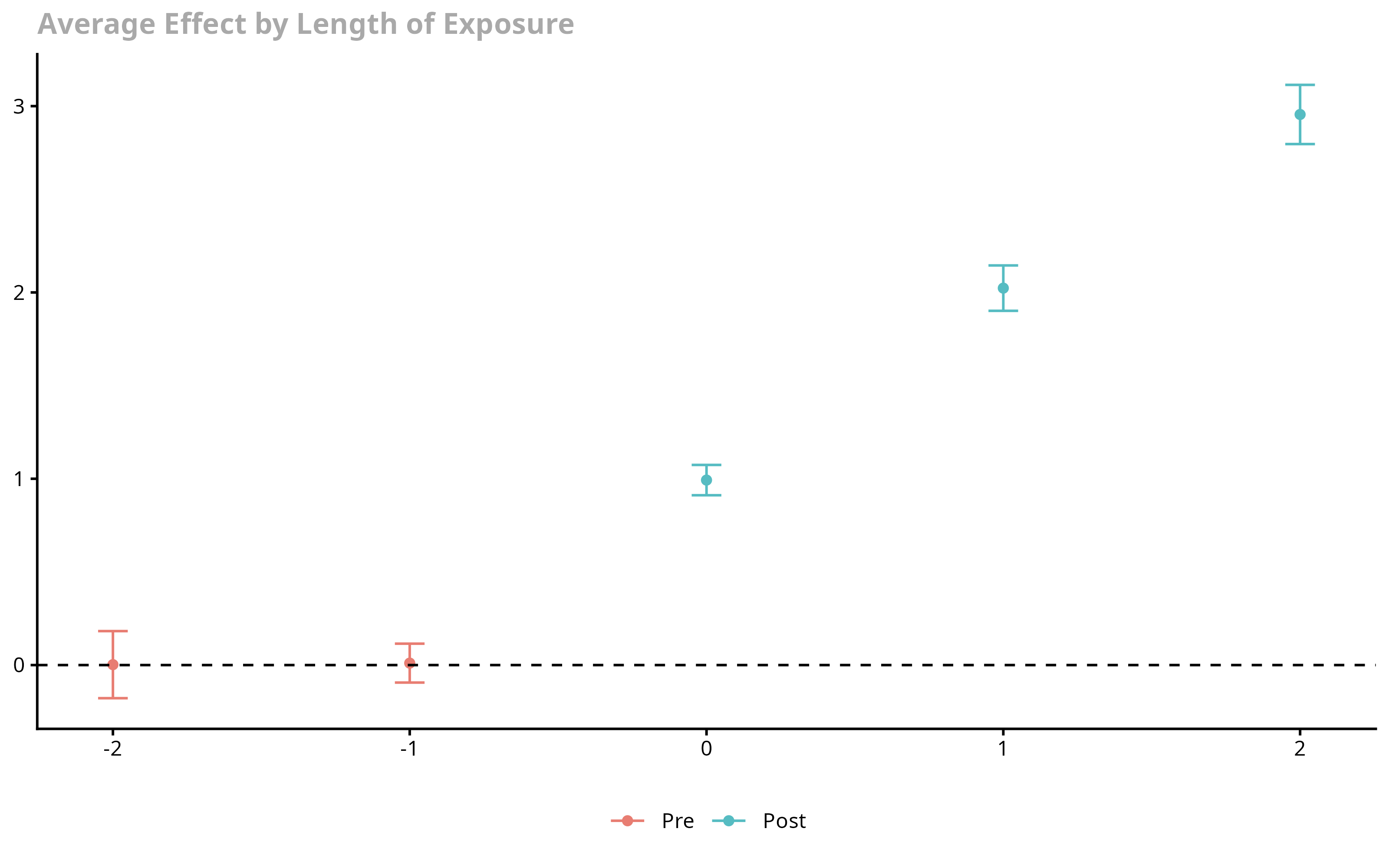
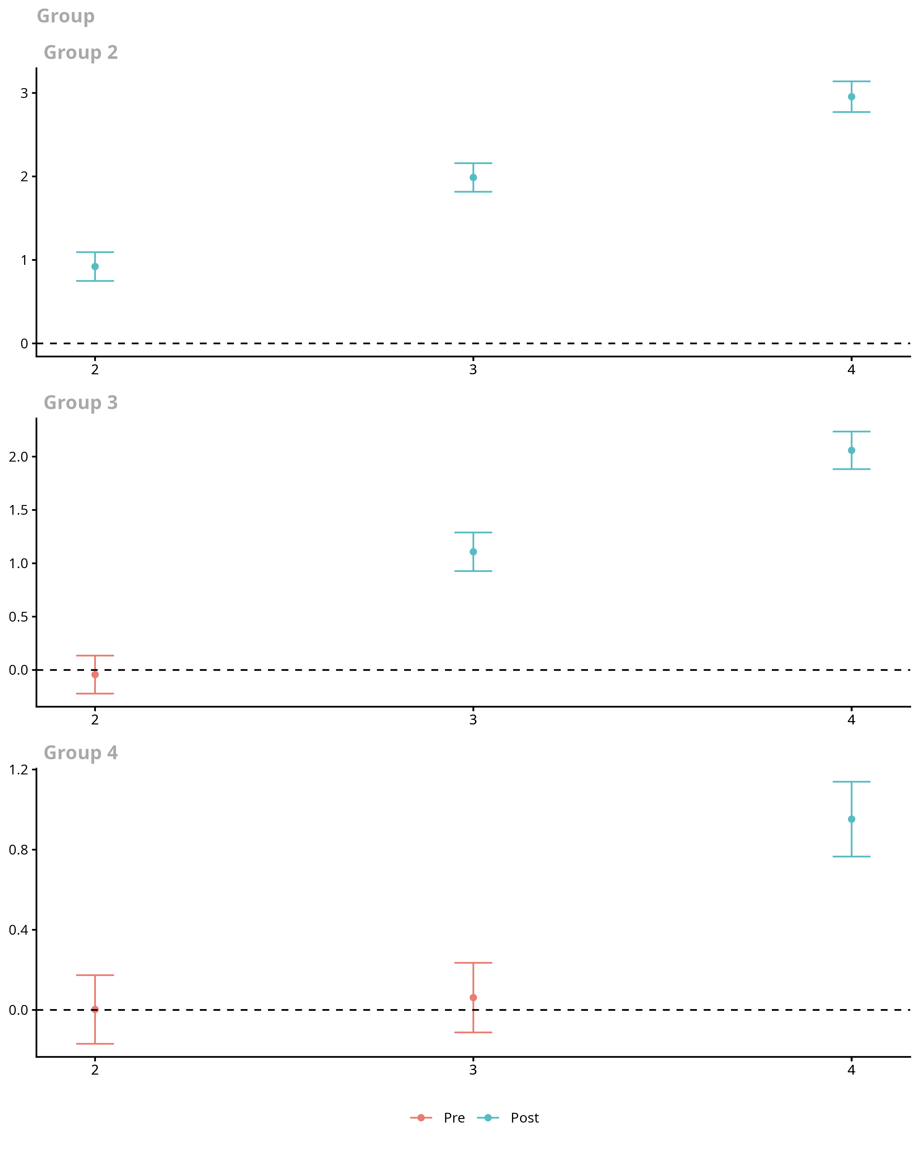
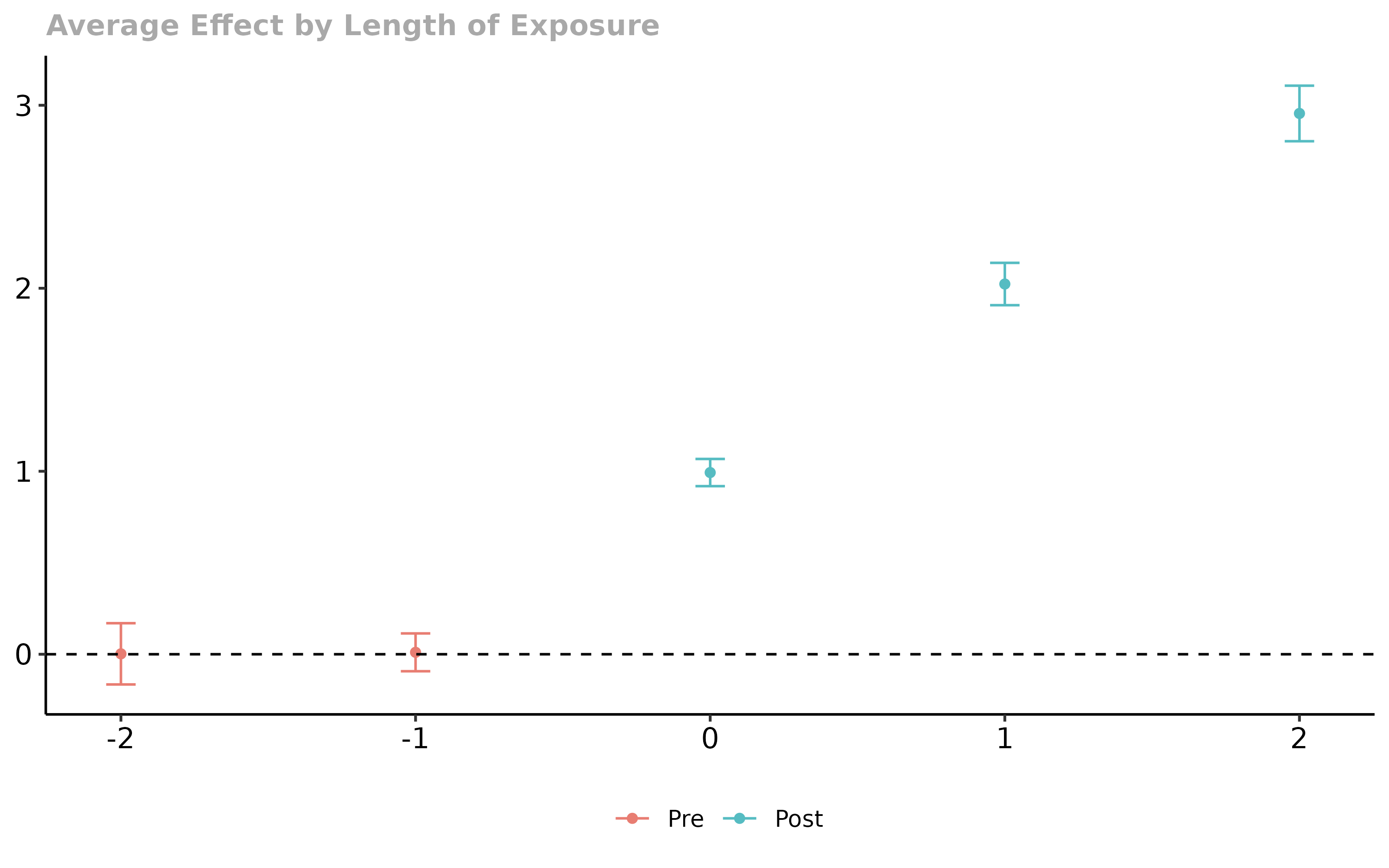
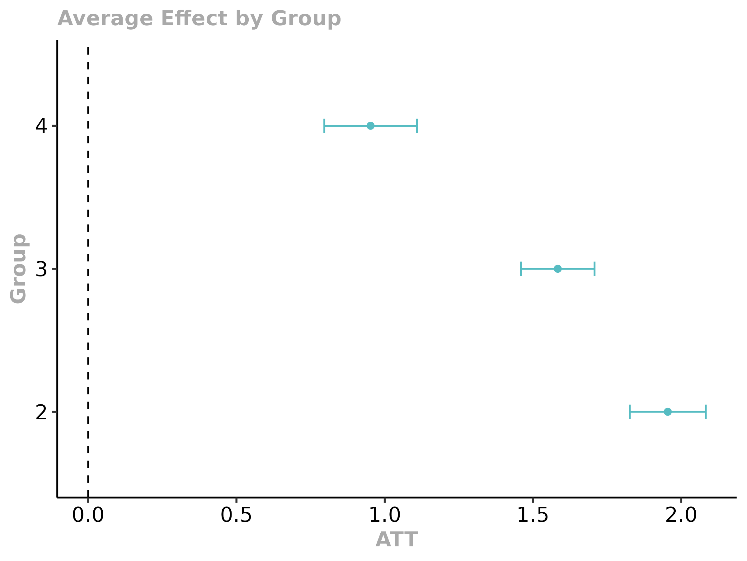
Staggered-adoption DiD done right: group-time ATT(g,t) → event-study / group / calendar aggregations, with honest pre-trends.
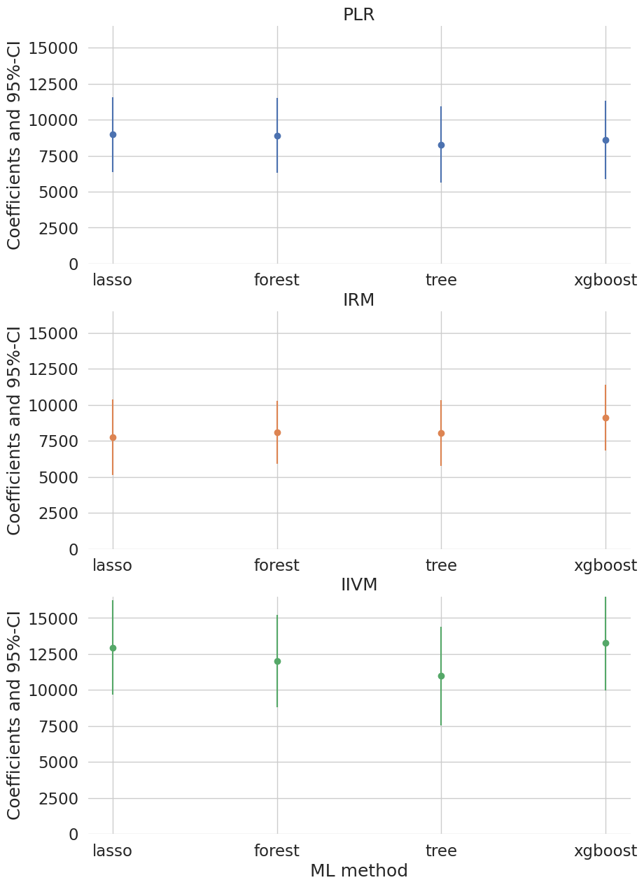
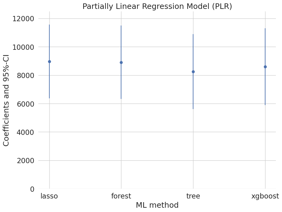
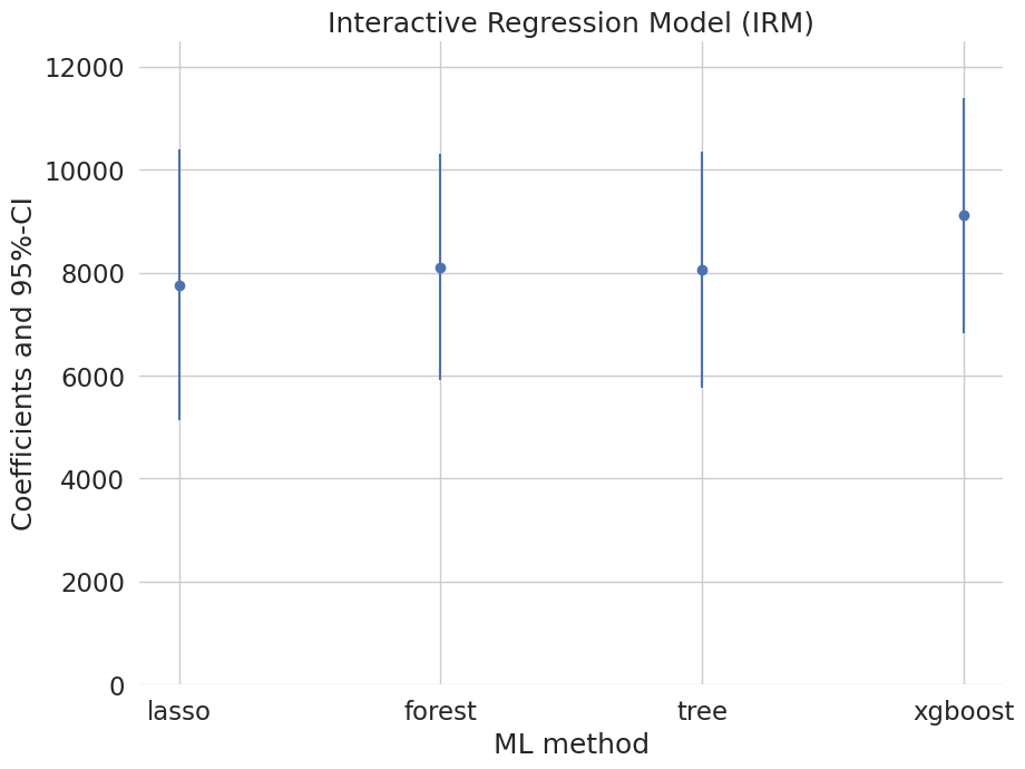
Effect of 401(k) eligibility on net assets via PLR / IRM / IIVM with cross-fit ML nuisances — four learners, one honest comparison.
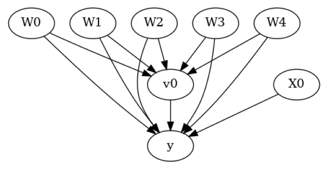
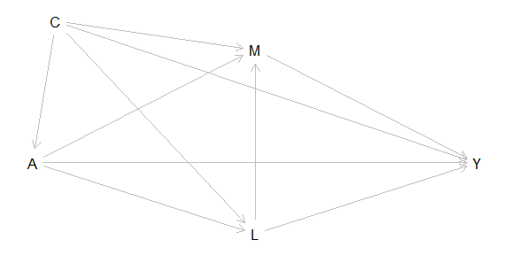
Make your assumptions explicit: draw a causal graph, identify the estimand by the backdoor criterion, estimate it, then actively try to refute it with placebo and confounding tests.
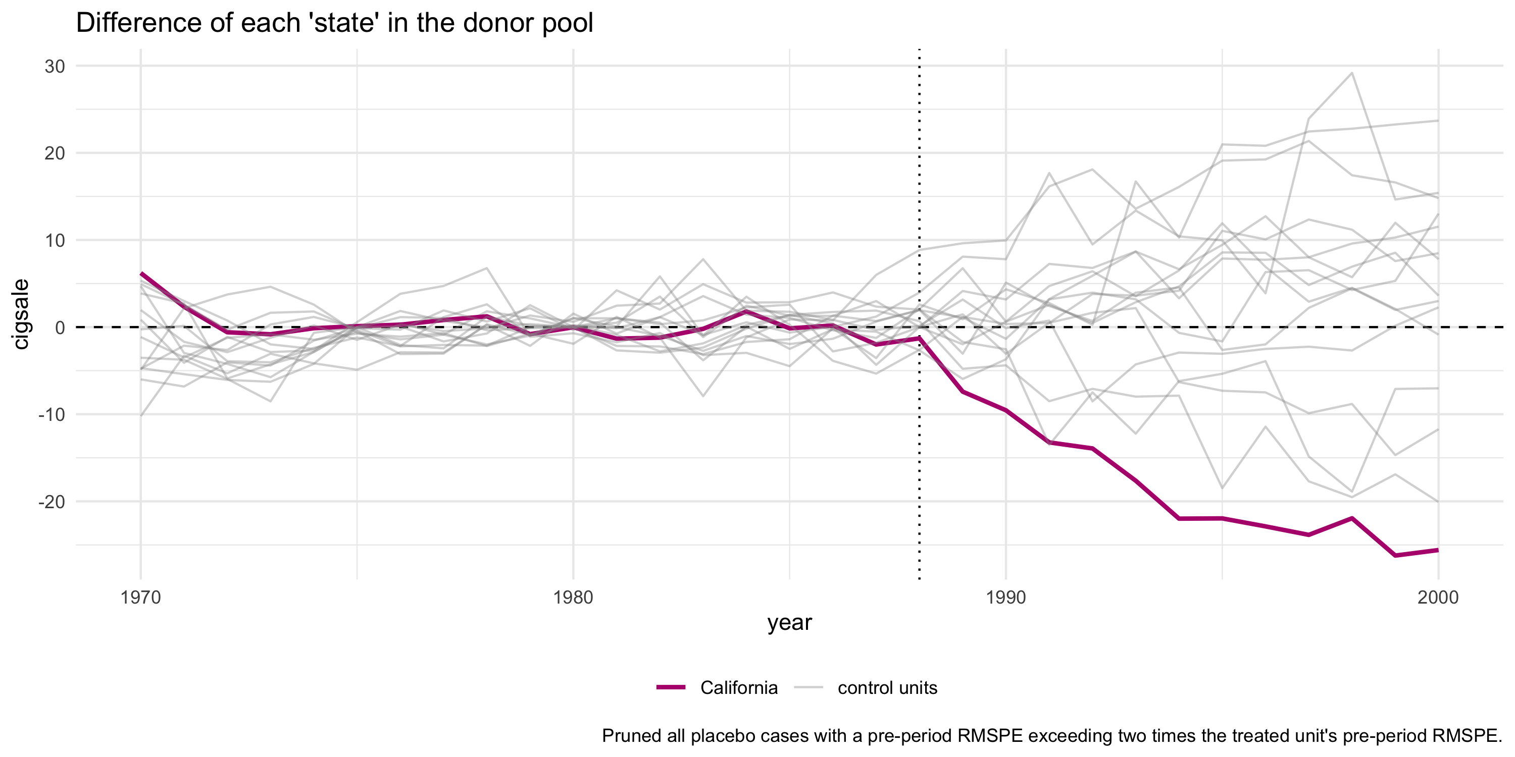
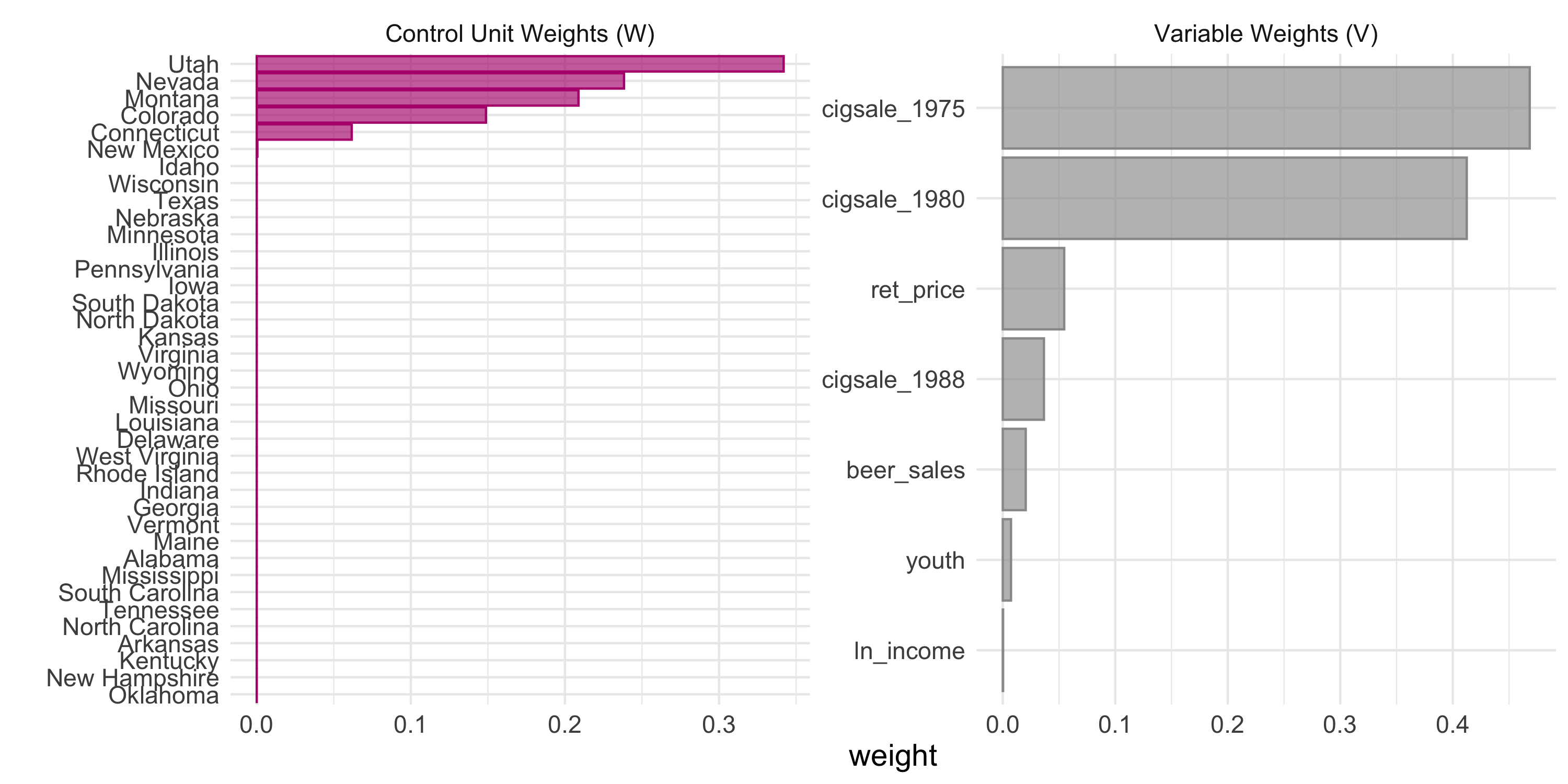
Build a synthetic version of the treated unit from a convex blend of donors, read the treated-minus-synthetic gap, and test it against placebos run on every donor.
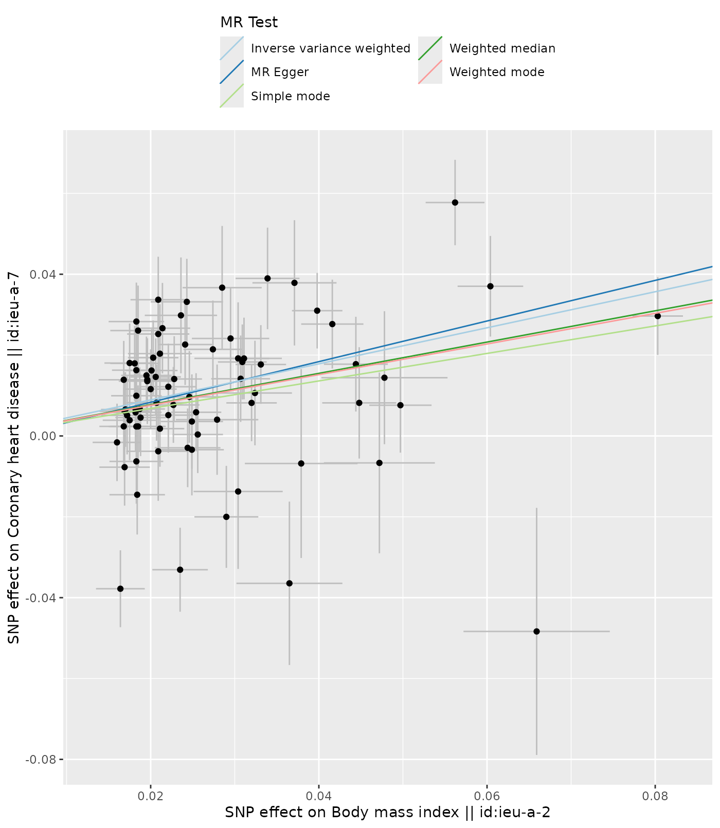
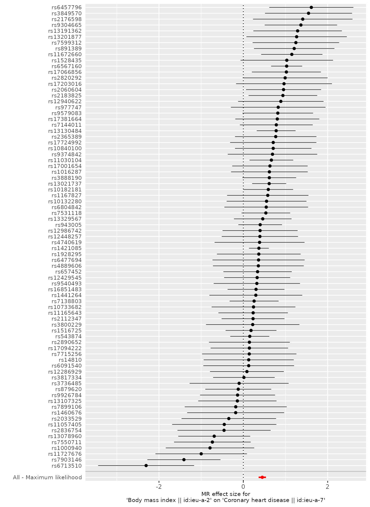
Use genetic variants as instruments to estimate the causal effect of an exposure on an outcome from GWAS summary data — with IVW plus pleiotropy-robust MR-Egger and weighted-median checks.
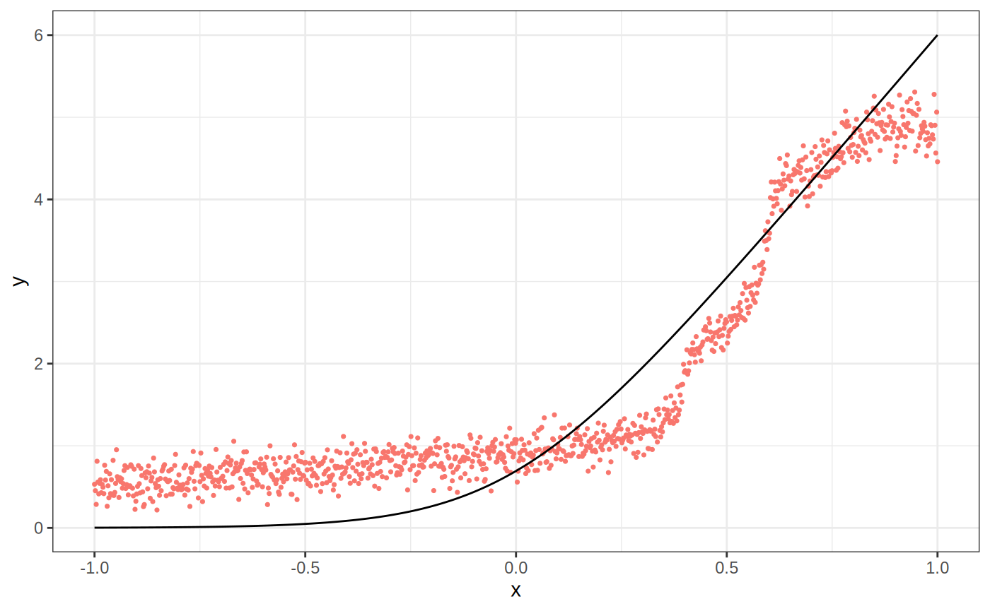
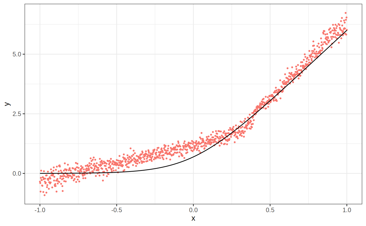
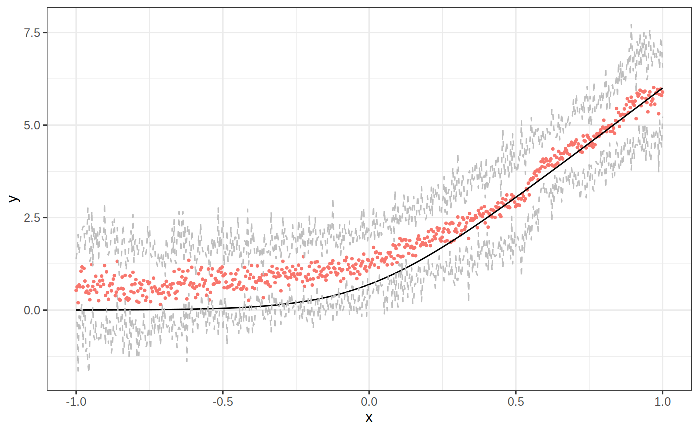
A minimal first-contact recipe: regression forest, quantile forest, and a causal forest on the same data.
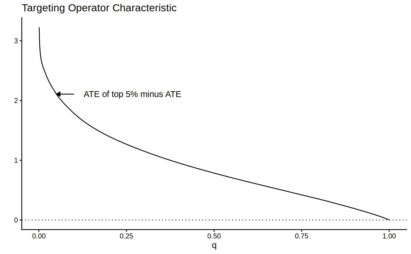
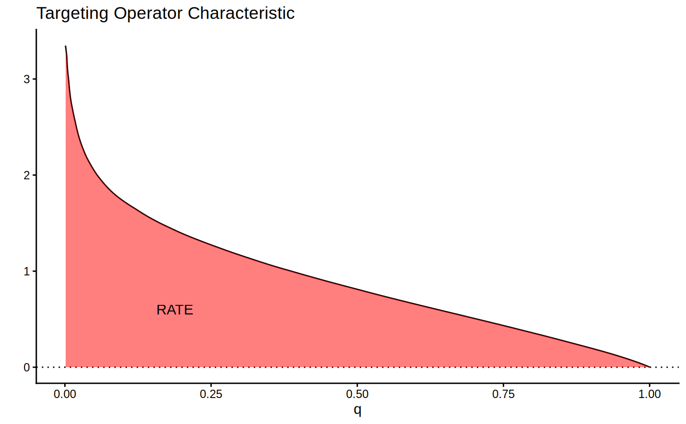
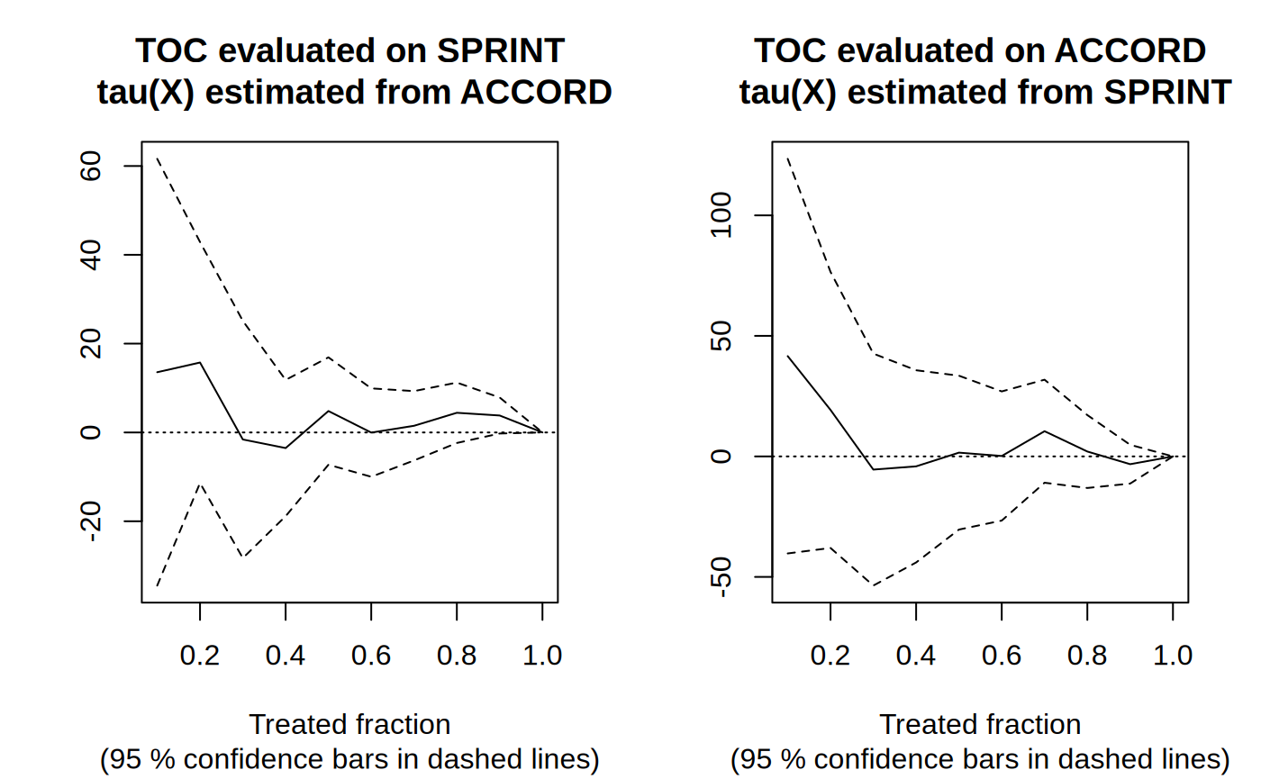
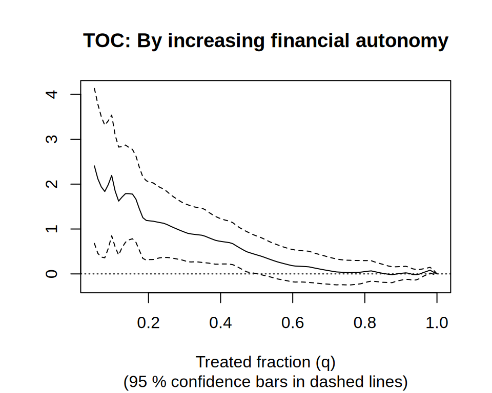
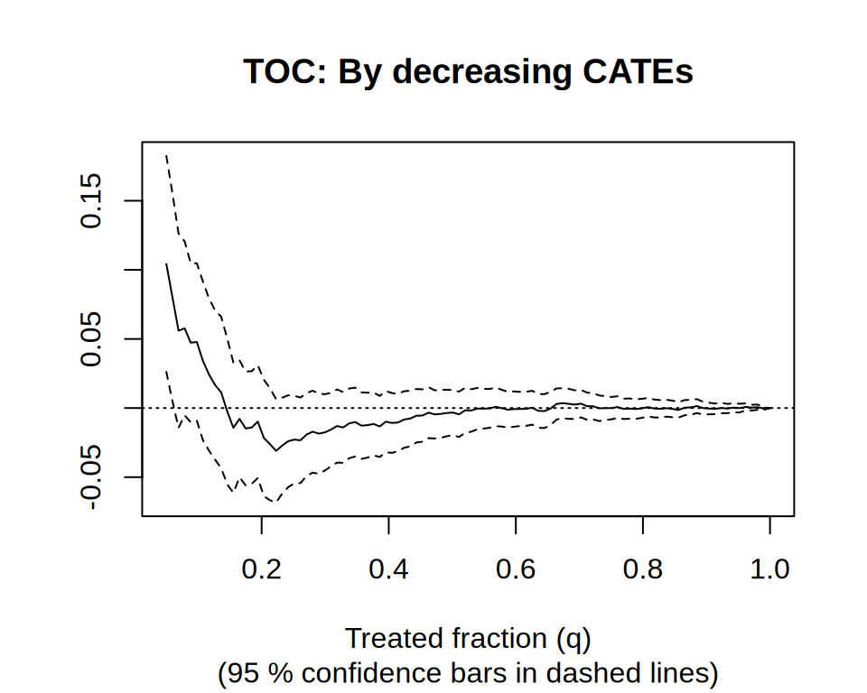
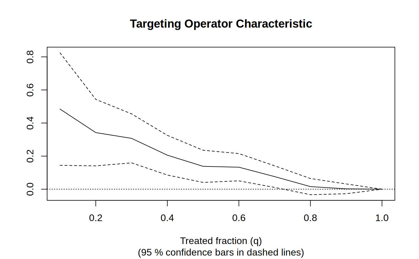
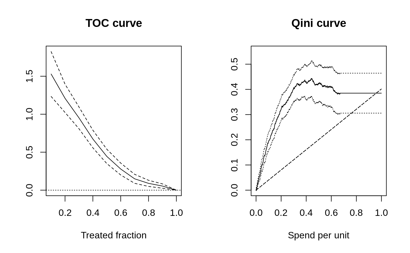
Causal forest → train/eval split → RATE with both AUTOC and Qini → TOC plot.
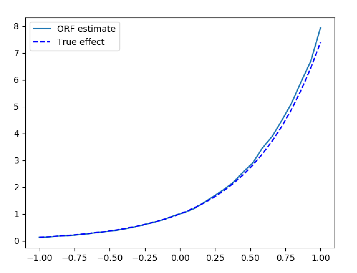
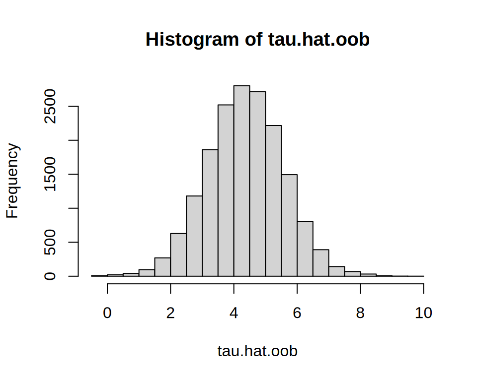
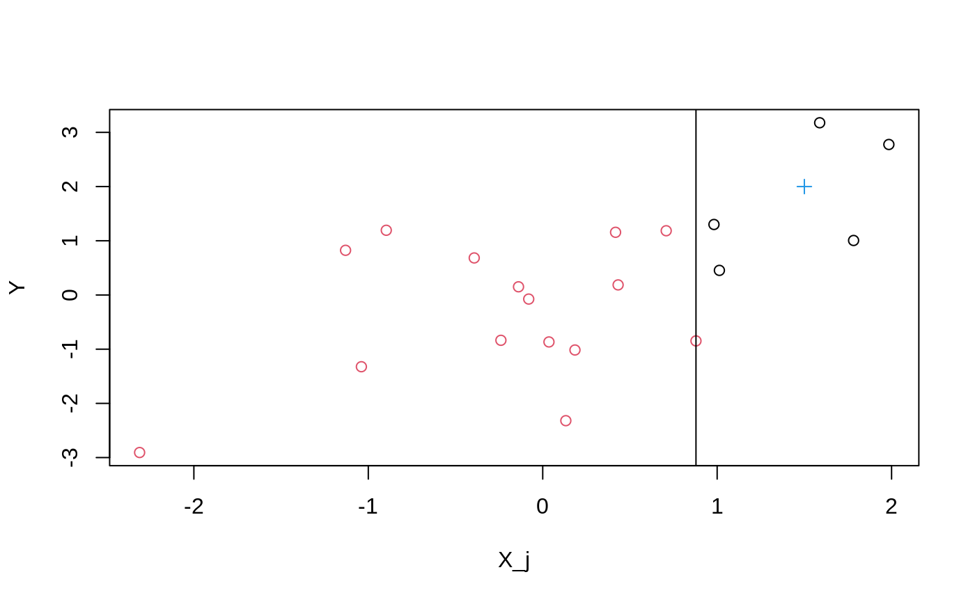
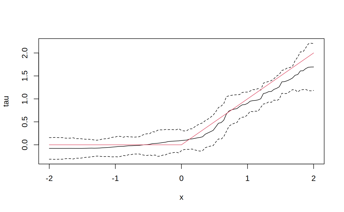
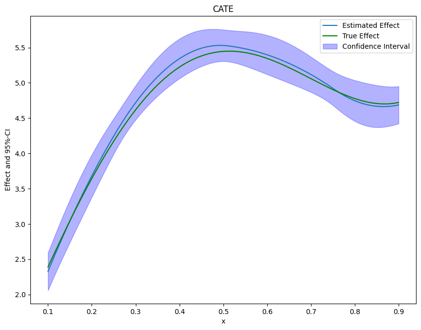
Double machine learning with a forest final stage: partial out nuisance with flexible learners, then read the conditional effect τ(x) — with valid confidence intervals.
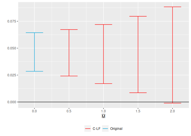
Stop betting everything on a pre-trends test. Allow the post-treatment trend to deviate within a transparent class, and report the confidence set — and the breakdown value where the effect would vanish.
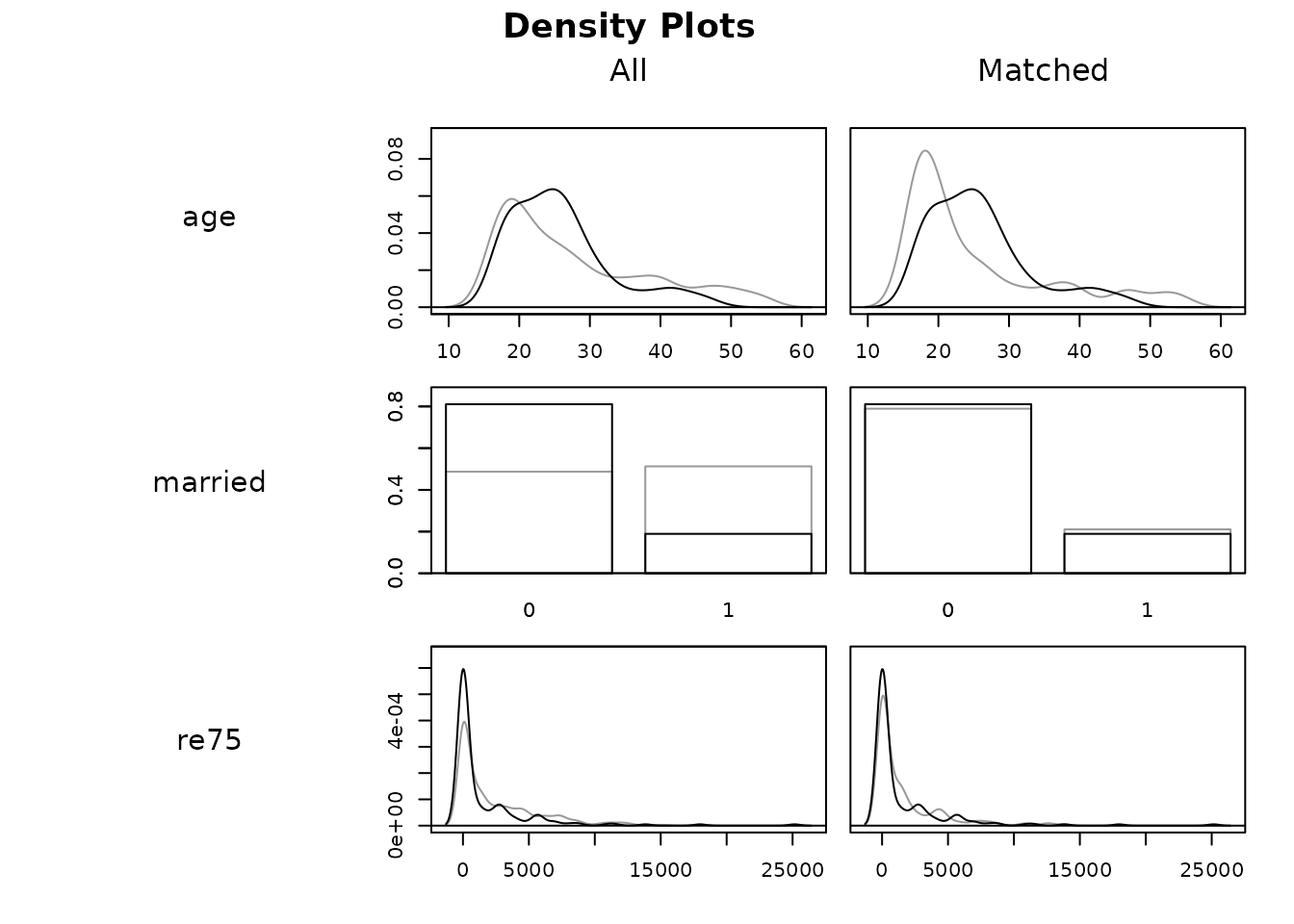

Preprocess by matching so groups are comparable, check balance, then estimate the effect on the matched sample — design before analysis.
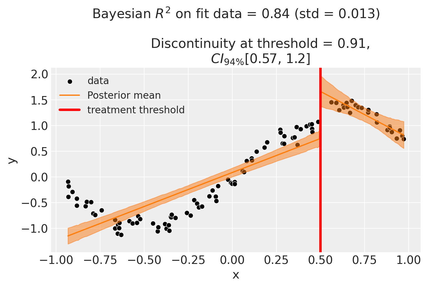
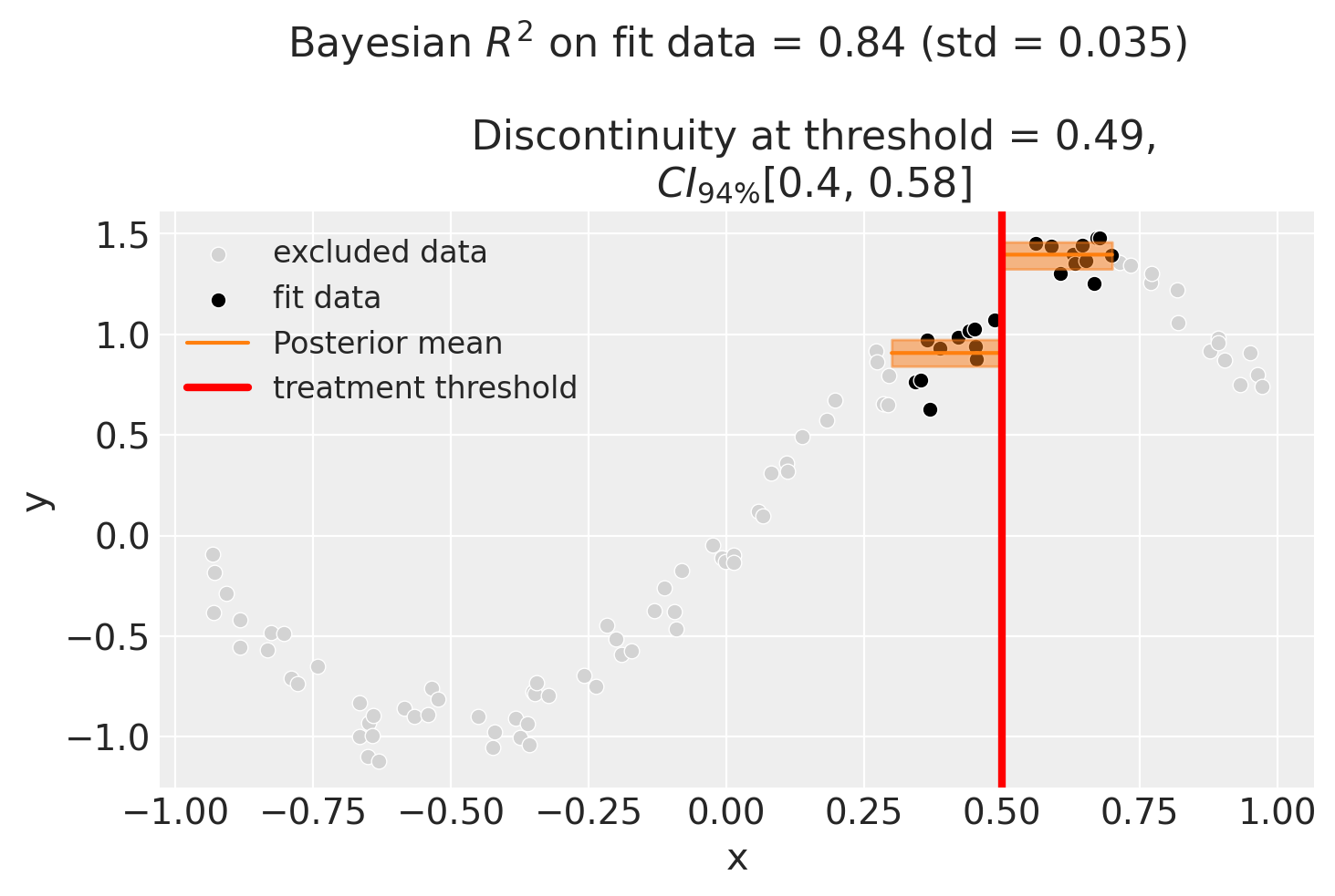
Fit a model on each side of the cutoff, put a posterior on the jump, and report a credible interval for the discontinuity — plus an honest look at how it moves with the bandwidth.

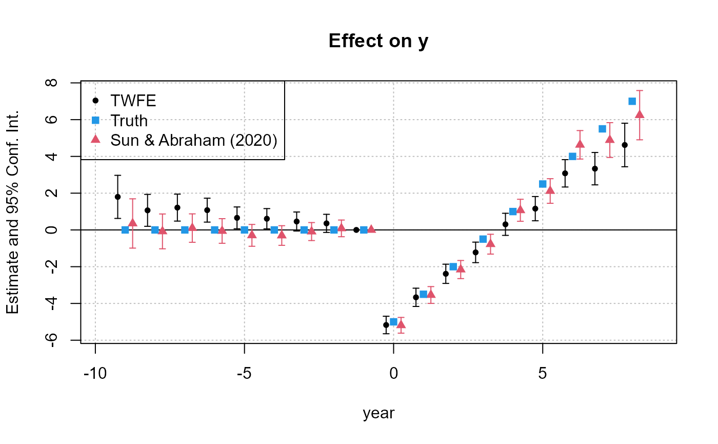
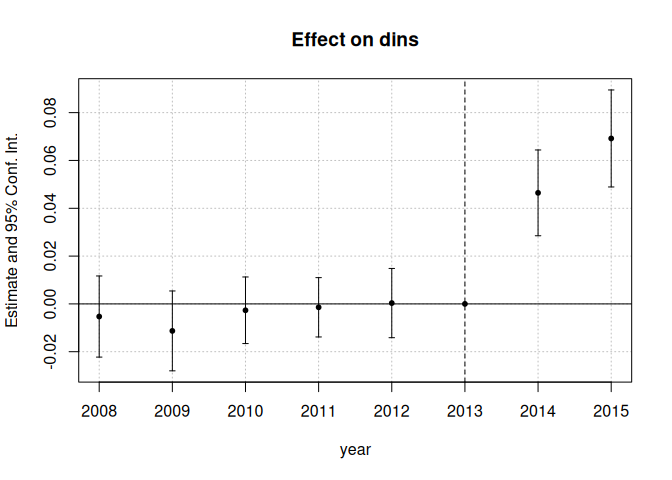
Fast fixed-effects event study that survives staggered timing — sunab() vs naive TWFE, plotted against the truth.

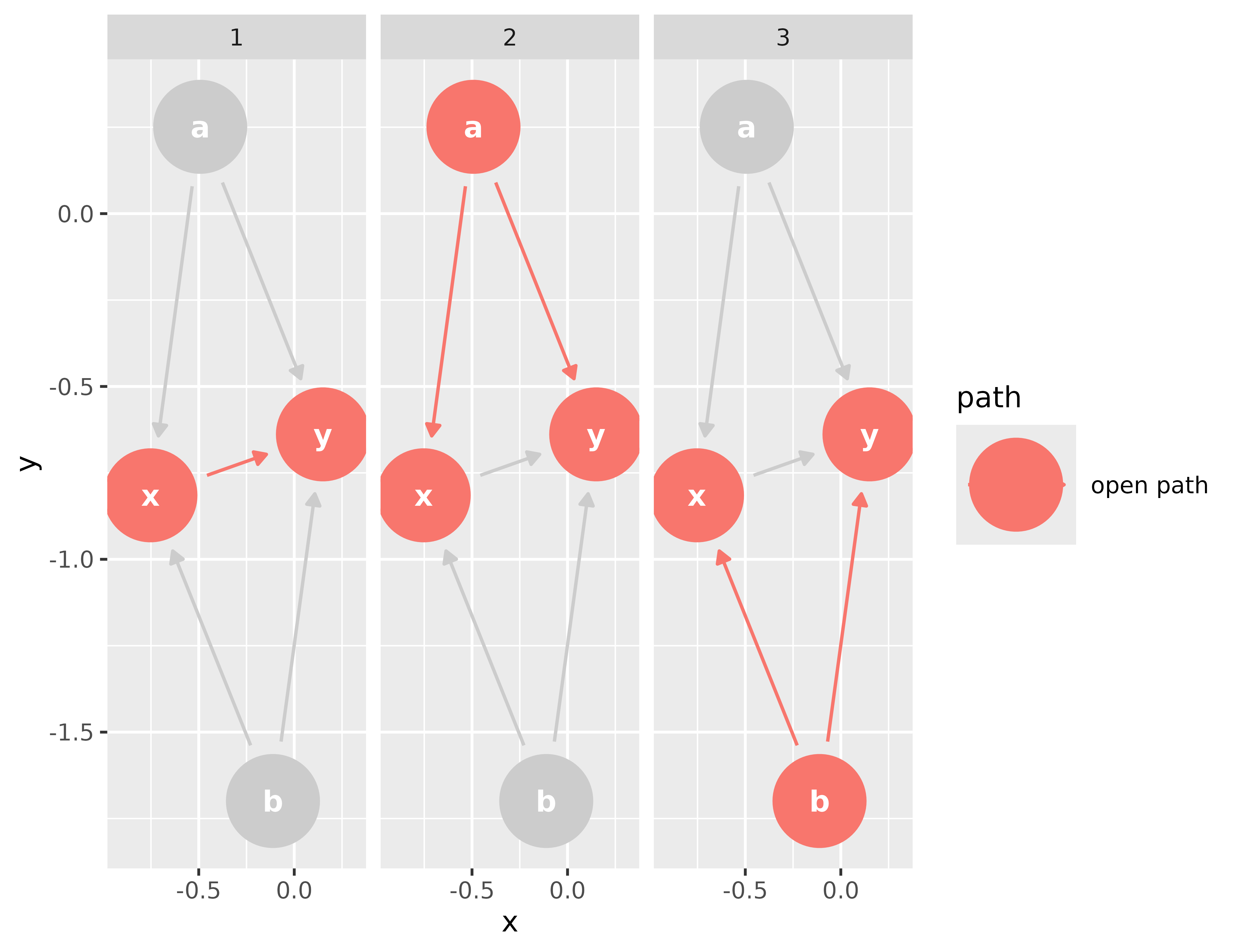
Before any estimation: encode your assumptions as a causal graph, enumerate the backdoor paths from treatment to outcome, and let the graph hand you the minimal set of covariates to adjust for.
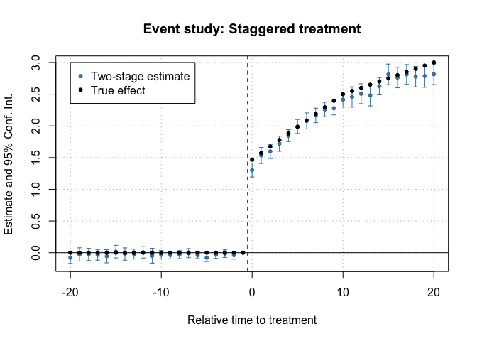
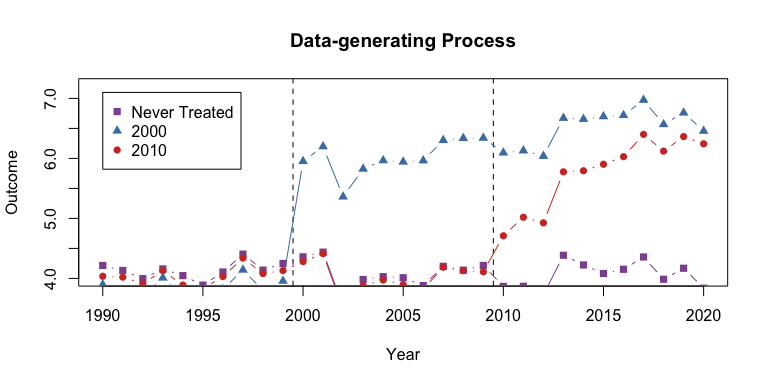
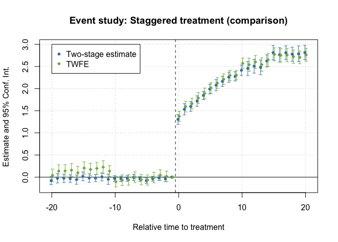
Gardner's 2-stage estimator for staggered DiD: residualize on the untreated, then estimate the event study — fast and timing-robust.
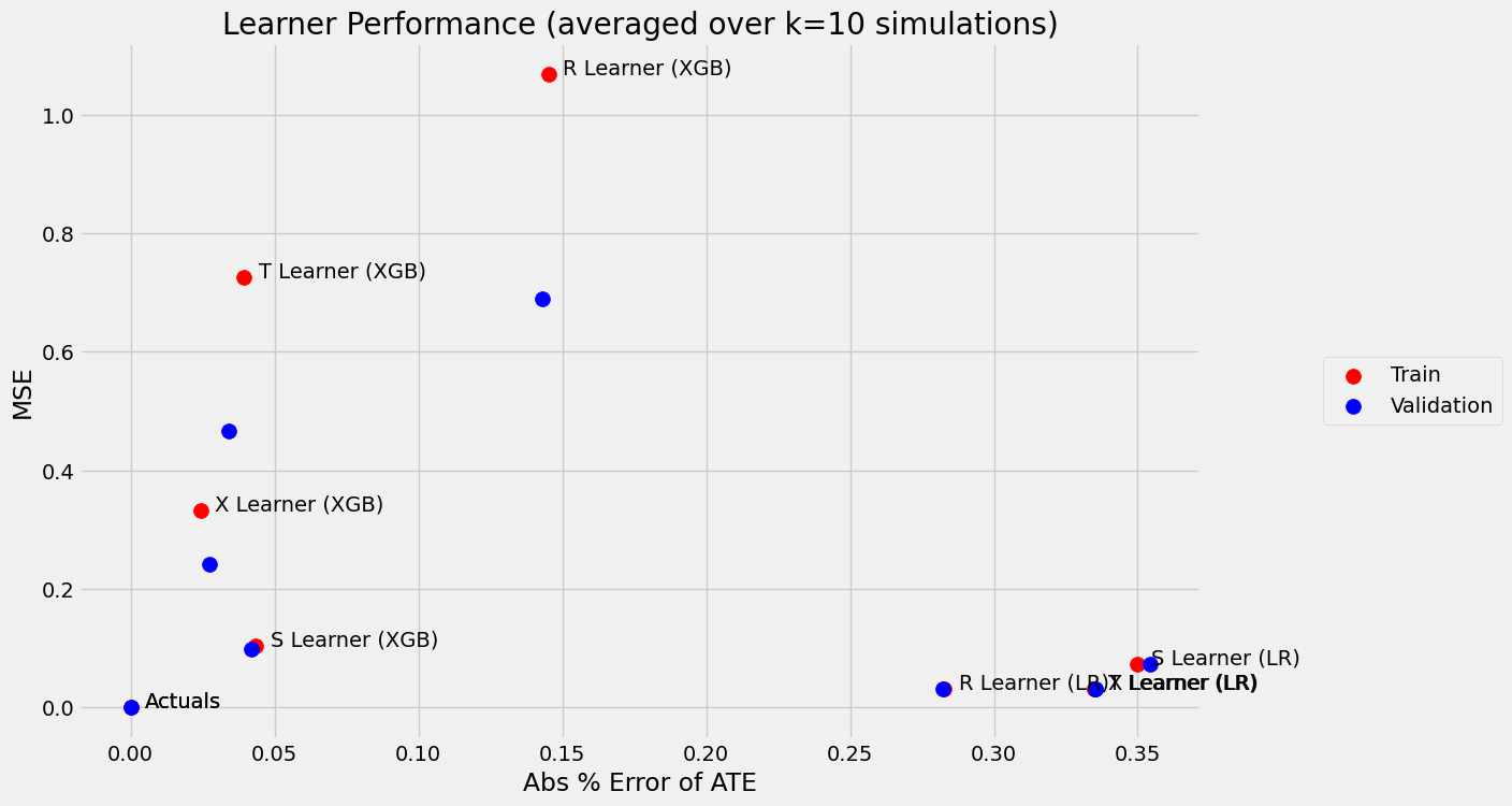
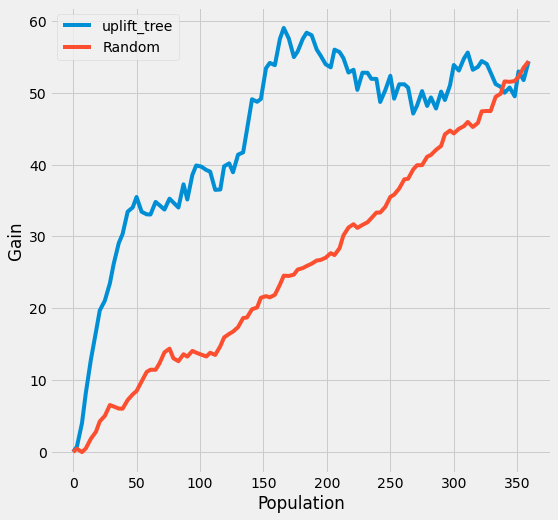
Estimate who responds, not just the average: fit a family of meta-learners for the CATE, pick the best by validation error, then rank and target with an uplift curve.
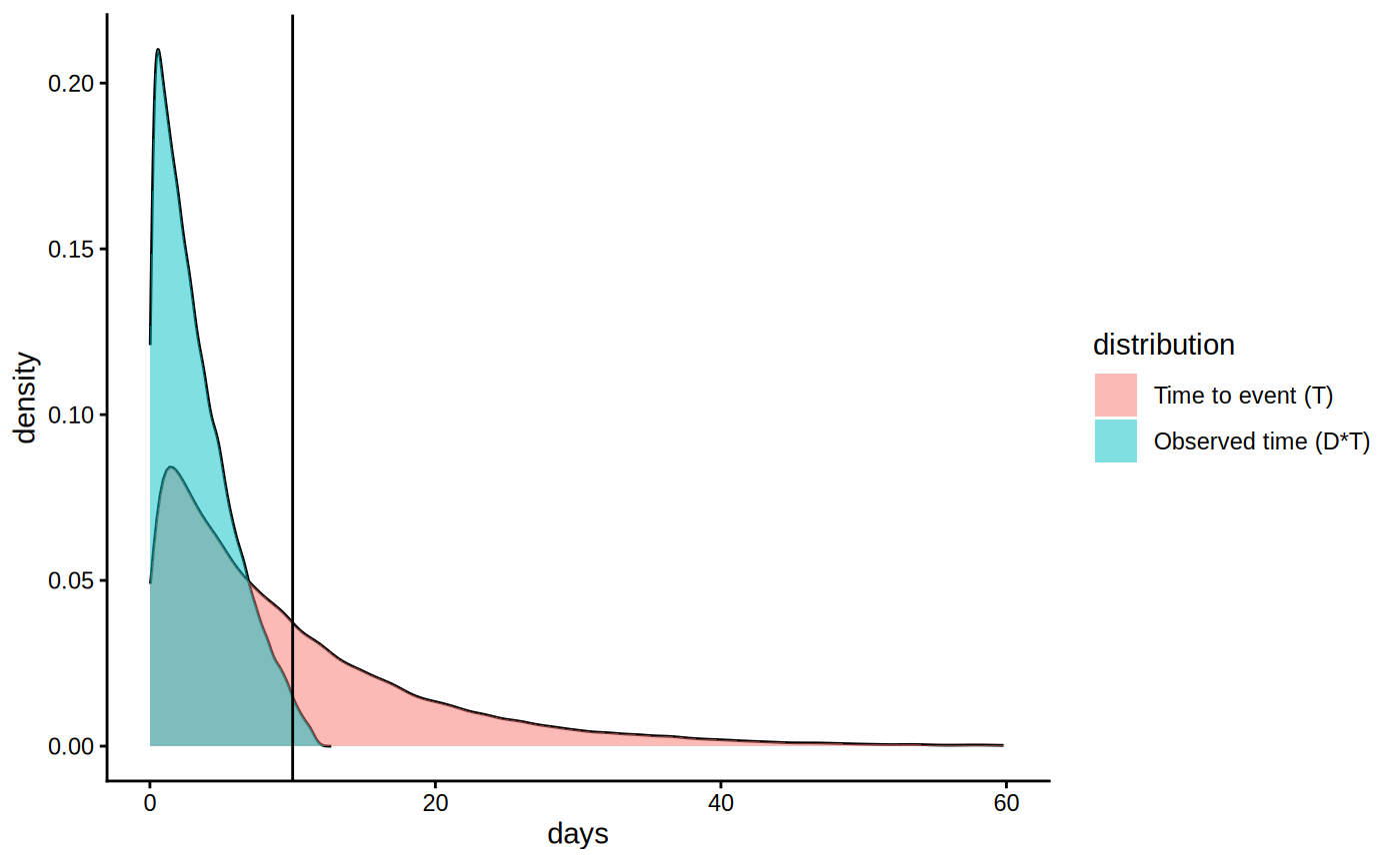
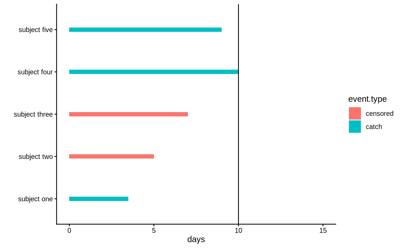
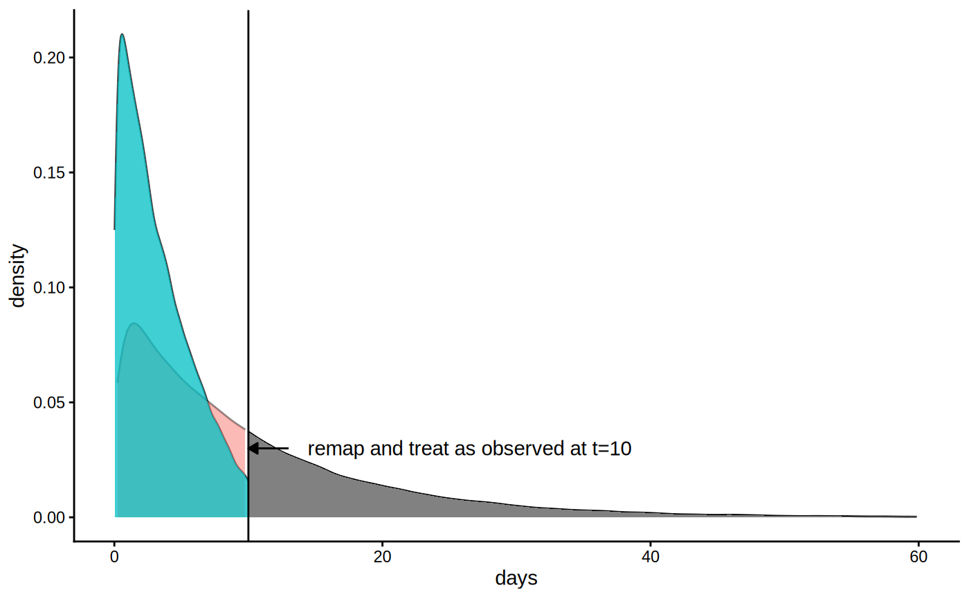
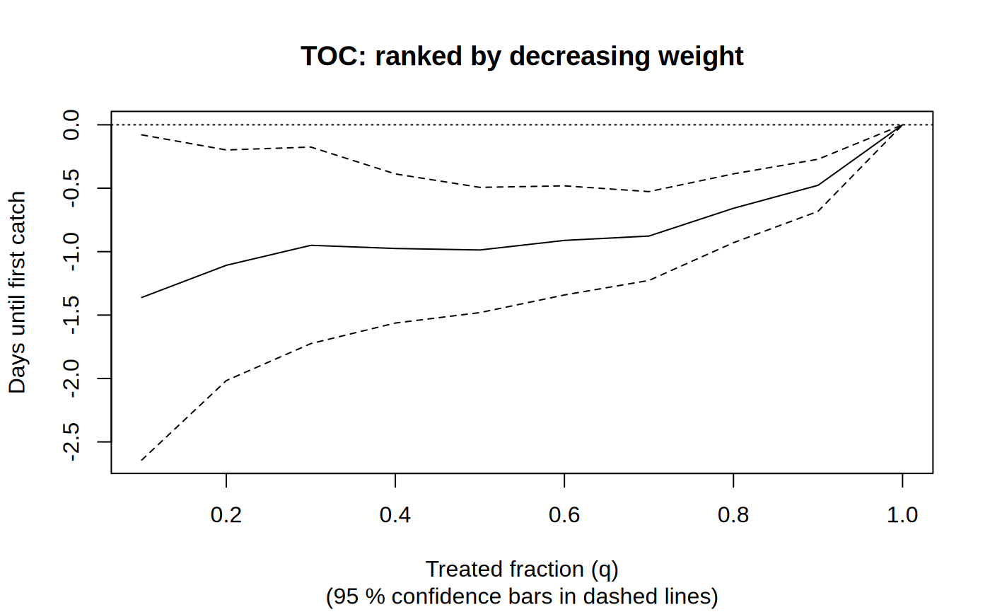
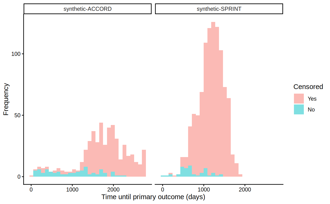
Censoring check → causal survival forest → RMST-scale AIPW ATE → calibration → report.
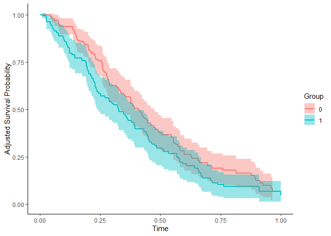
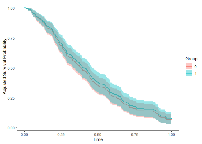
Compare survival between treatment groups after removing confounding — via IPTW, the g-formula or AIPW — instead of a raw Kaplan-Meier that quietly bakes in selection.
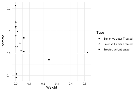
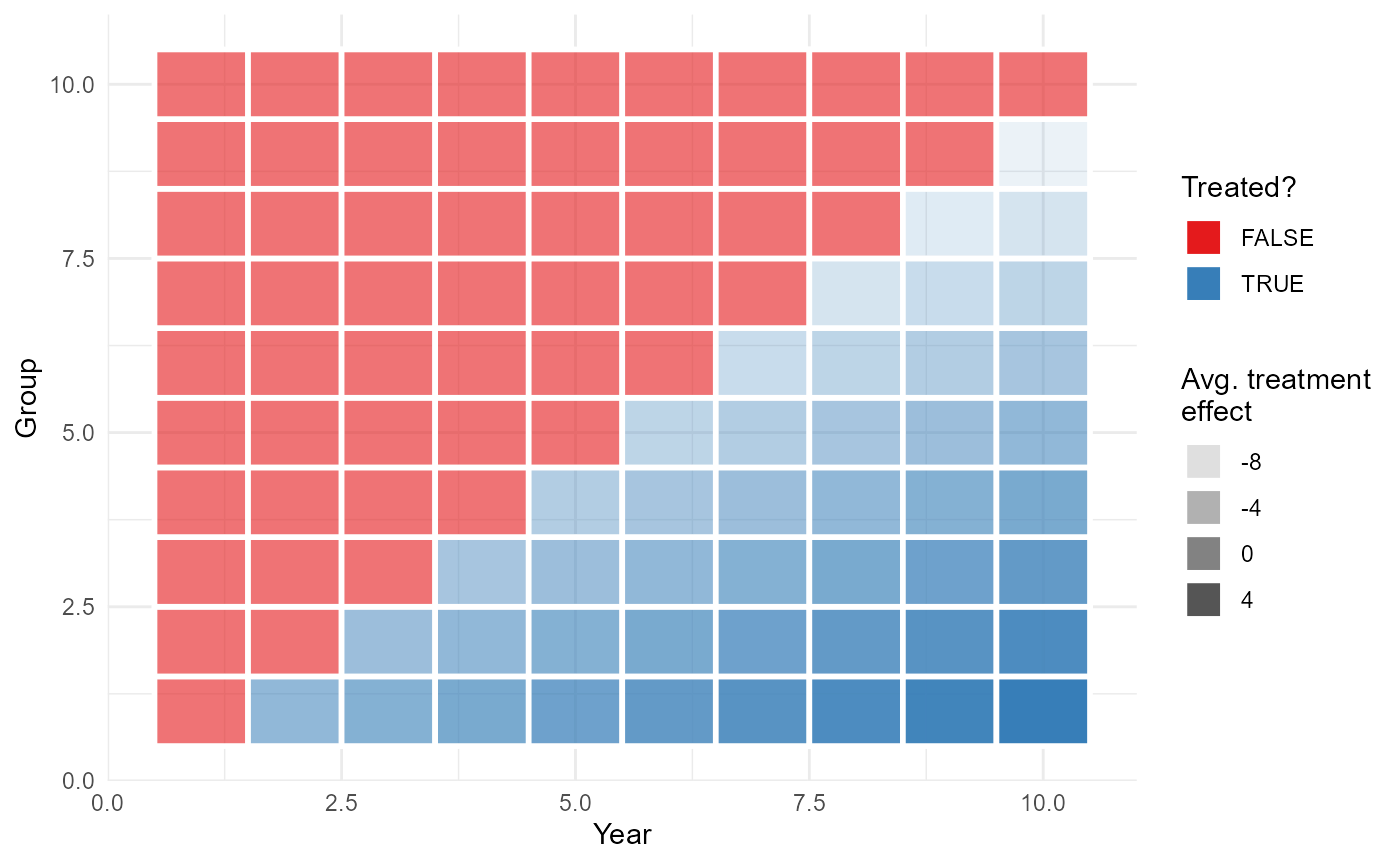
A two-way fixed-effects DiD is a weighted average of all possible 2×2 comparisons — including 'forbidden' ones that use already-treated units as controls. This shows you the weights.
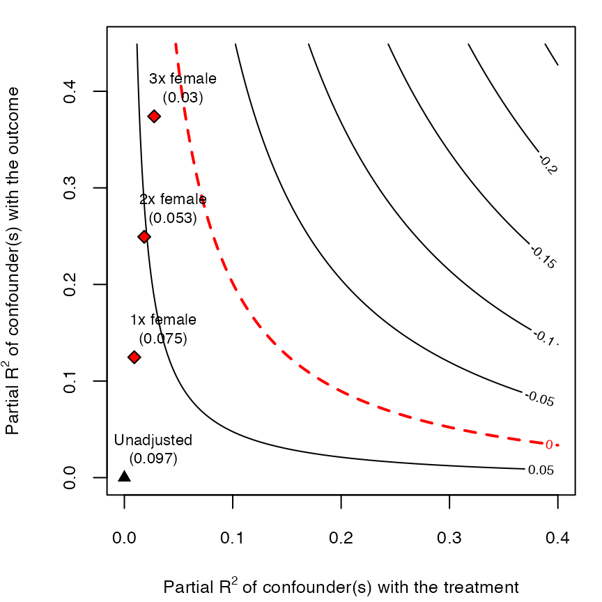
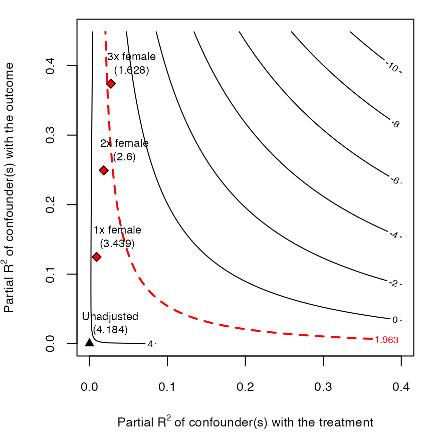
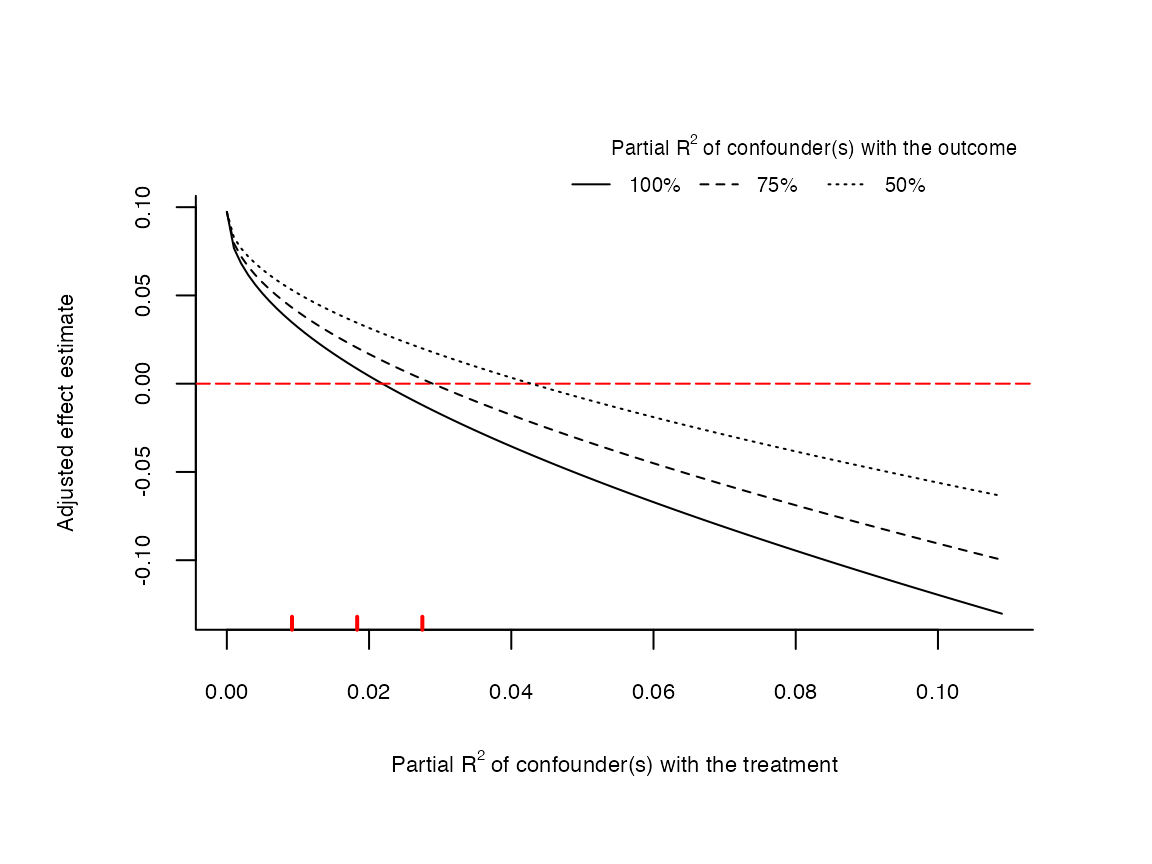
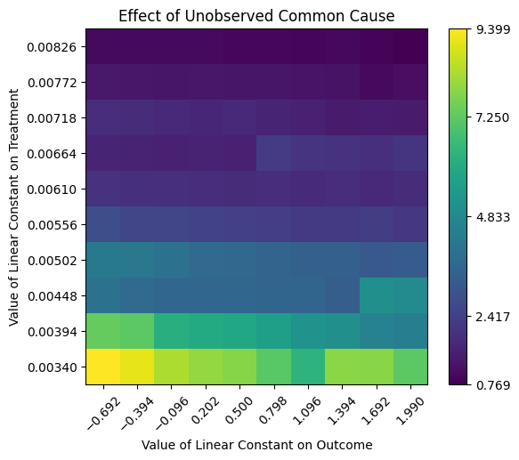
Don't just assume no unobserved confounding — quantify it: robustness value + contour plots benchmarked against your real covariates.
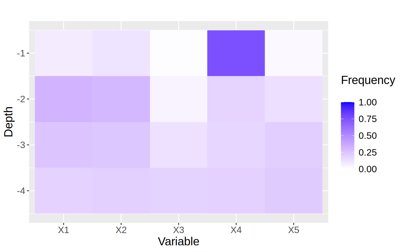
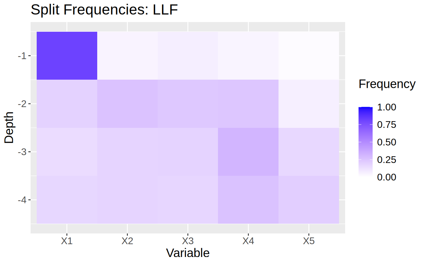
Did the forest actually capture treatment-effect heterogeneity? Calibration → variable importance → BLP → omnibus tests.
Specify a study as model–inquiry–data–answer, simulate it, and read its diagnosands — bias, power, coverage — before you run it.
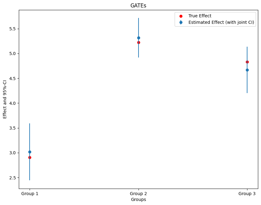
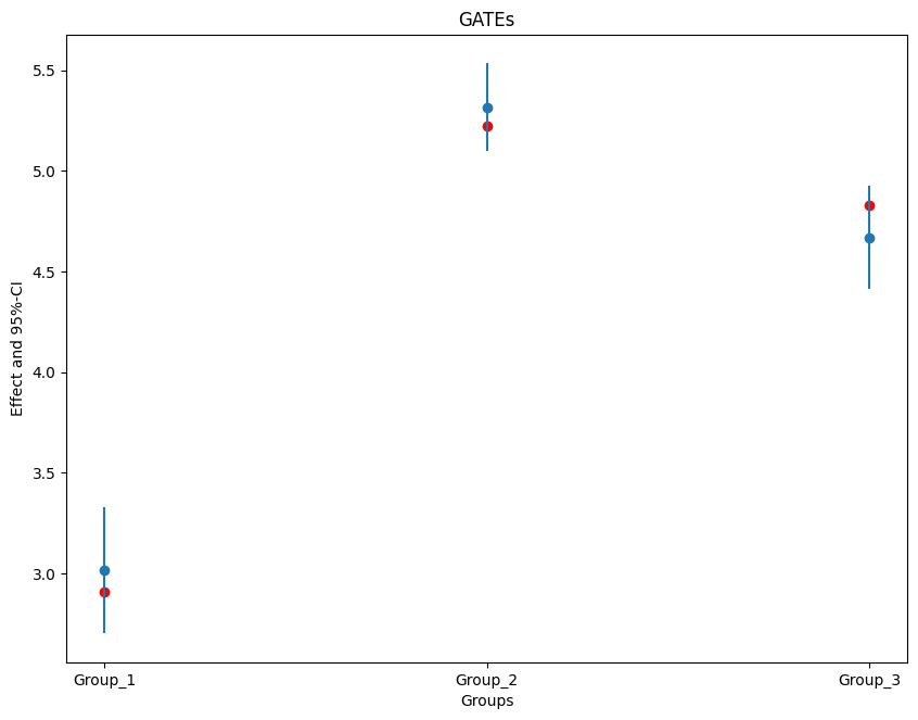
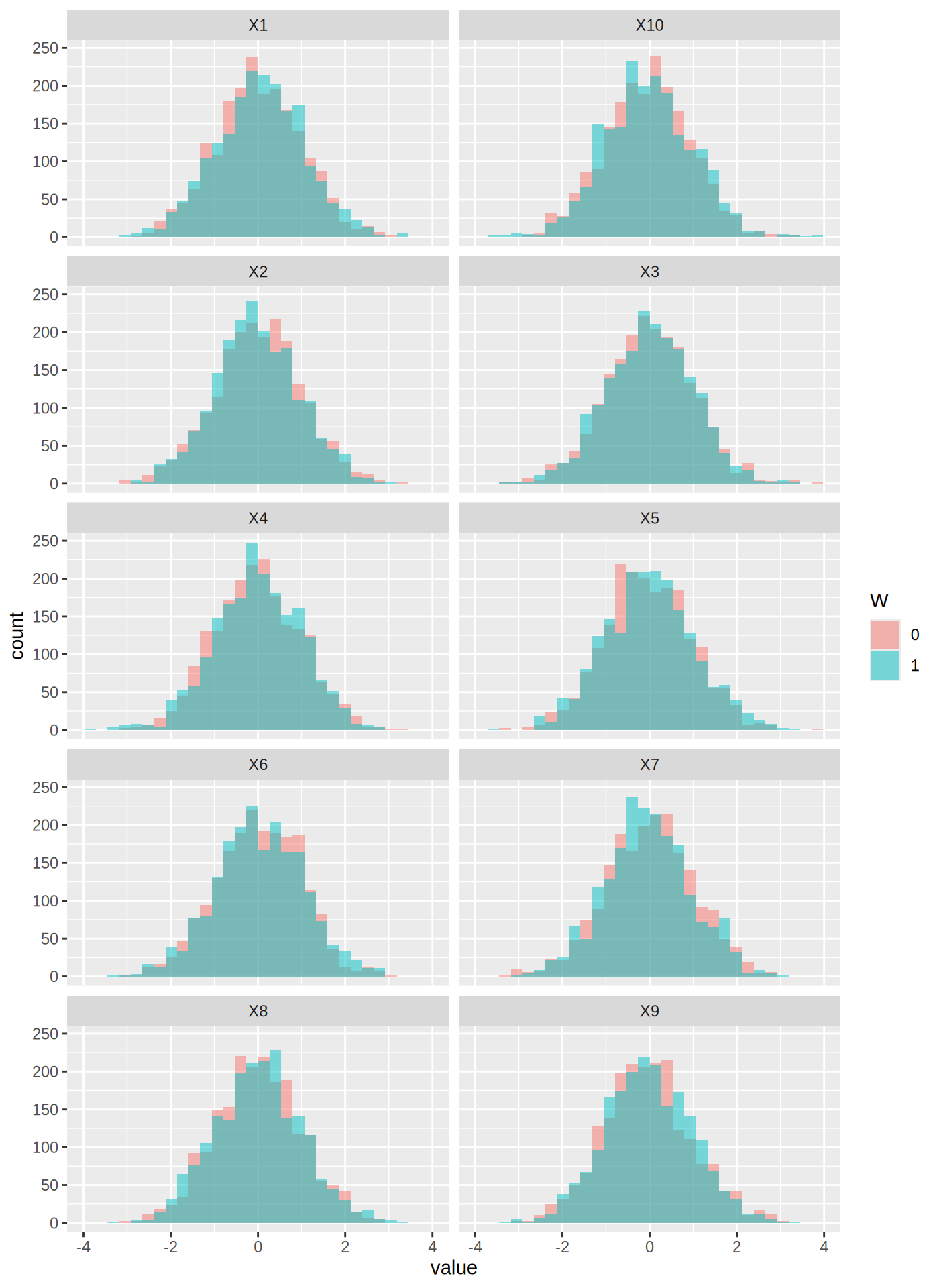
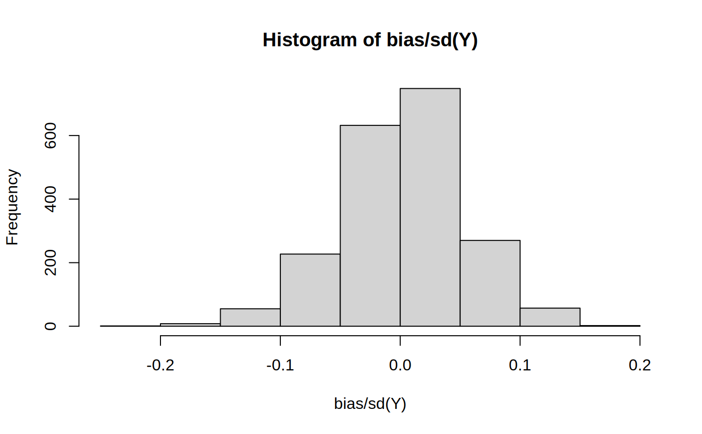
Slice the average effect: Group Average Treatment Effects and a CATE surface from a debiased IRM, with simultaneous confidence bands.
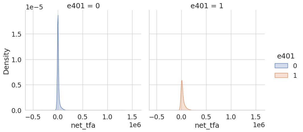
Beyond the average: how 401(k) eligibility shifts net financial assets across the whole wealth distribution, estimated orthogonally.
Identify the effect at a cutoff: a local-polynomial RD with an MSE-optimal bandwidth and robust, bias-corrected confidence intervals.
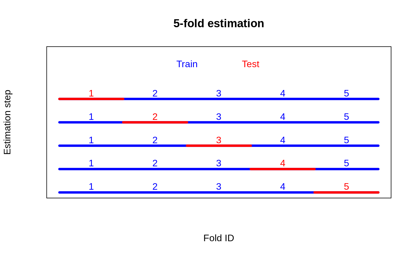
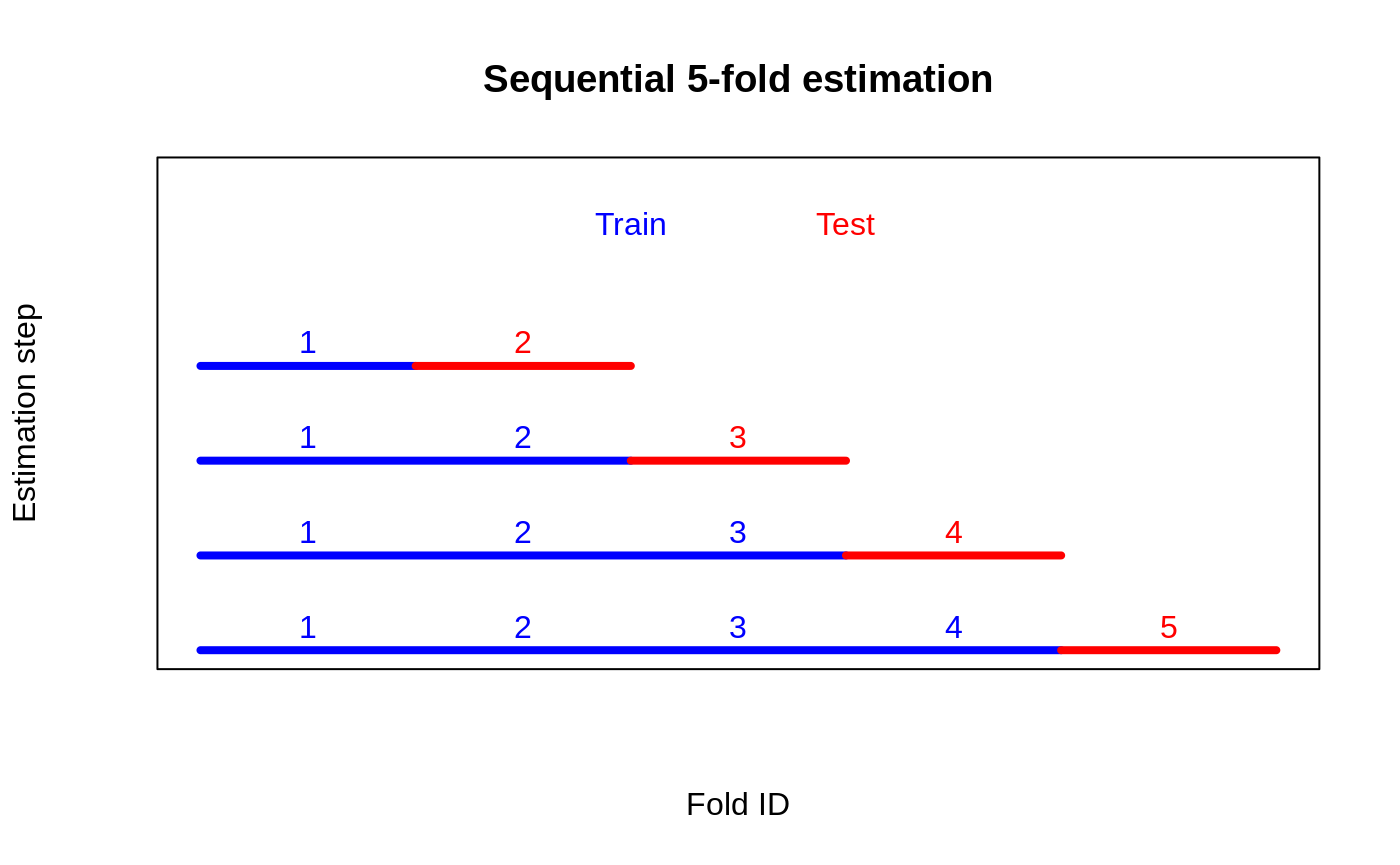
K-fold cross-fitted CATEs → RATE on out-of-fold priorities → honest verdict on heterogeneity strength.
Causal forest → doubly-robust scores → policytree → evaluate policy value → plot the tree.
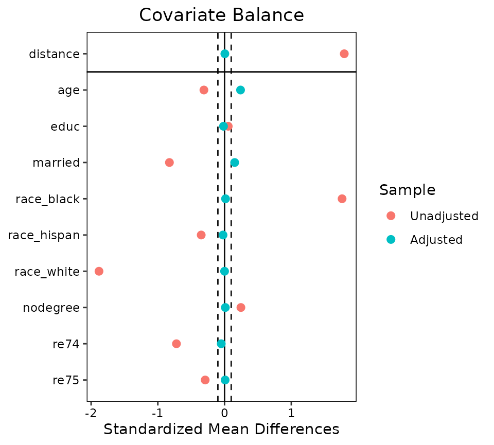
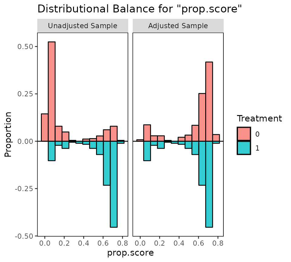
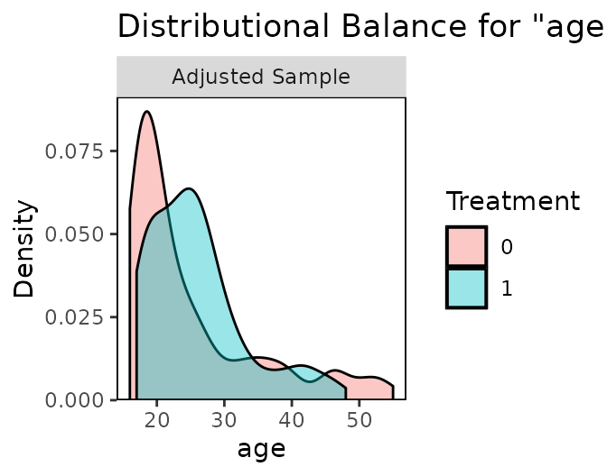
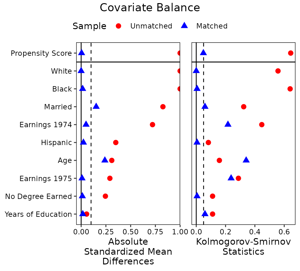
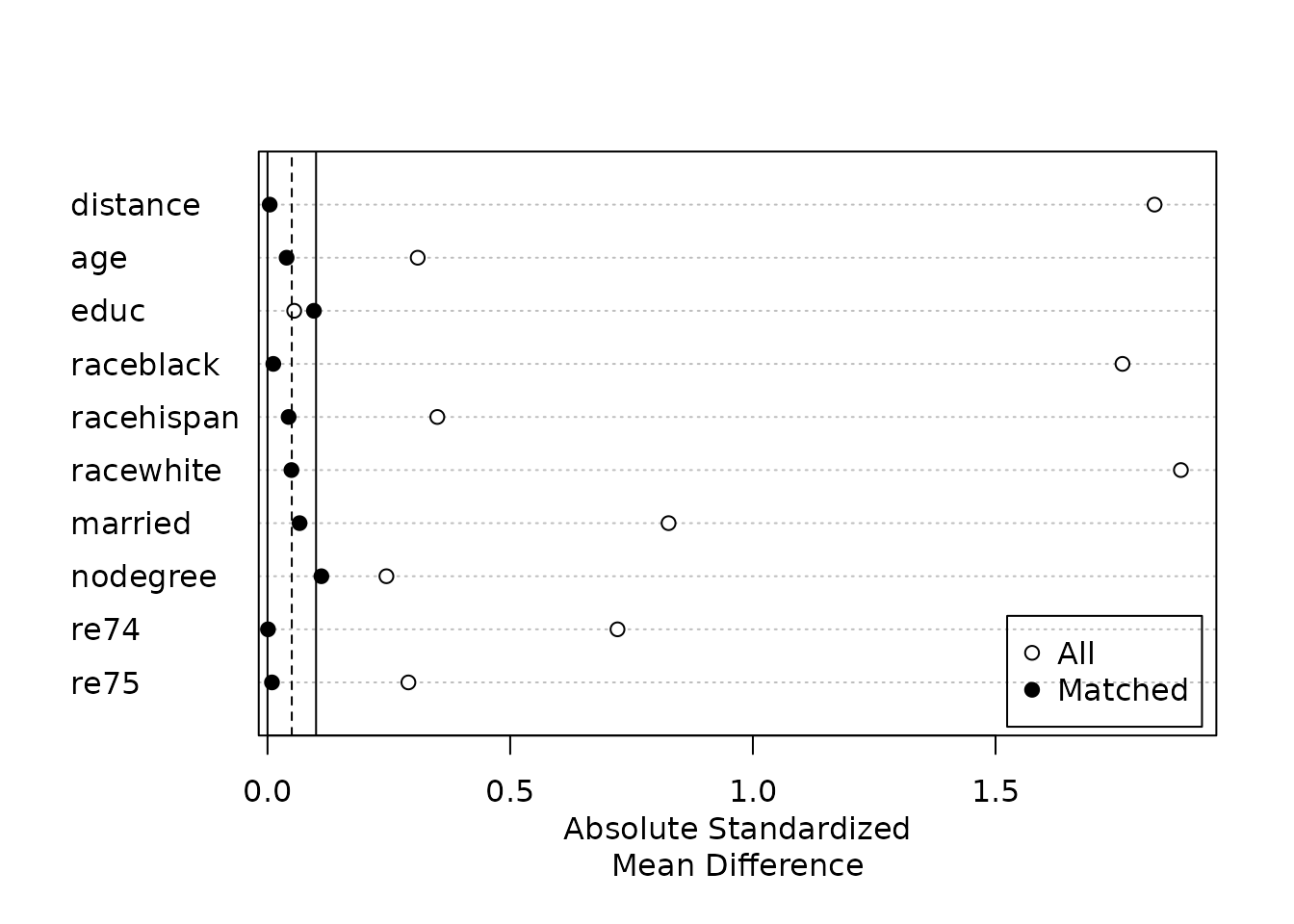
Before you trust an observational estimate, prove balance: SMDs, overlap, and a Love plot before vs after adjustment.
When the conditional mean is smooth: regression forest baseline → ll_regression_forest → tuning → diagnostics.
Reweight both control units and pre-periods to build a synthetic control, then apply a DiD correction — robust where plain SC or TWFE struggle.

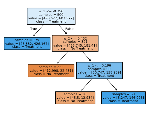
Turn debiased CATEs into a rule: fit a shallow, readable decision tree that maximises the doubly-robust policy value.
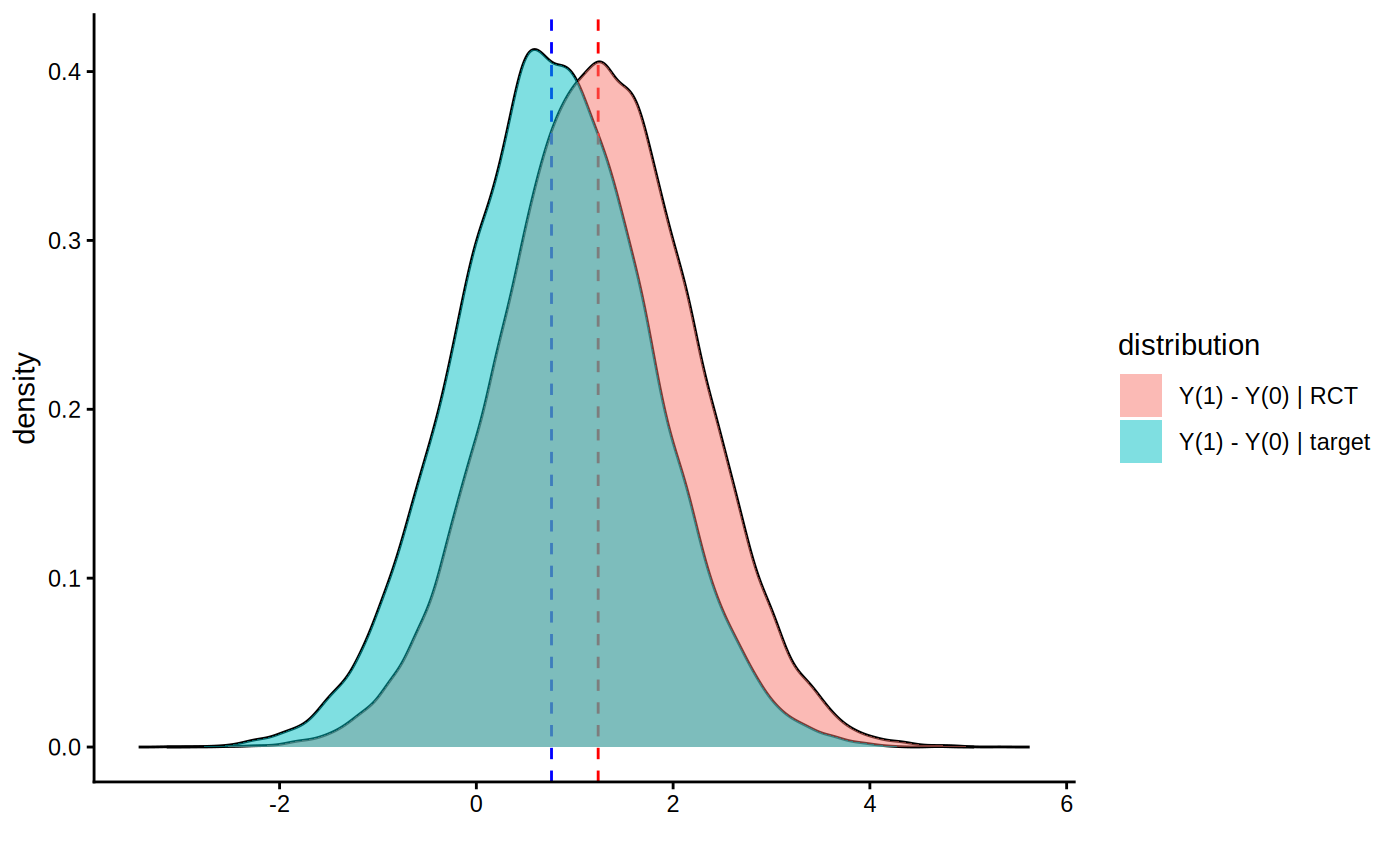
Train a causal forest on the source sample → reweight AIPW to a target population → report transported ATE.
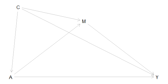
Split a total effect into what flows through a mediator (indirect) and what doesn't (direct) — with a sensitivity analysis for mediator–outcome confounding.
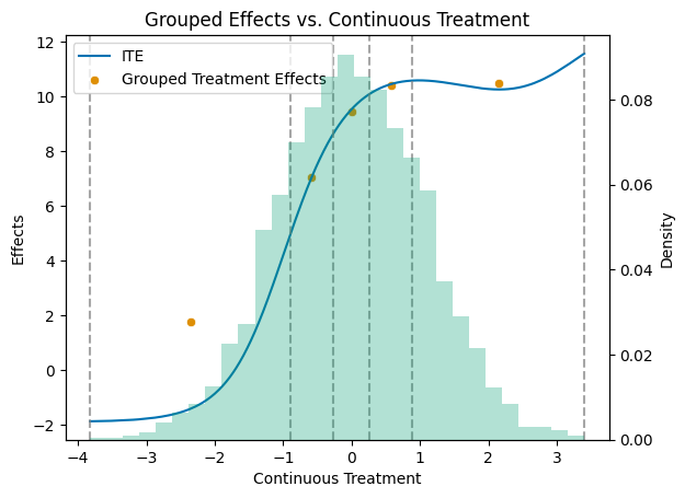
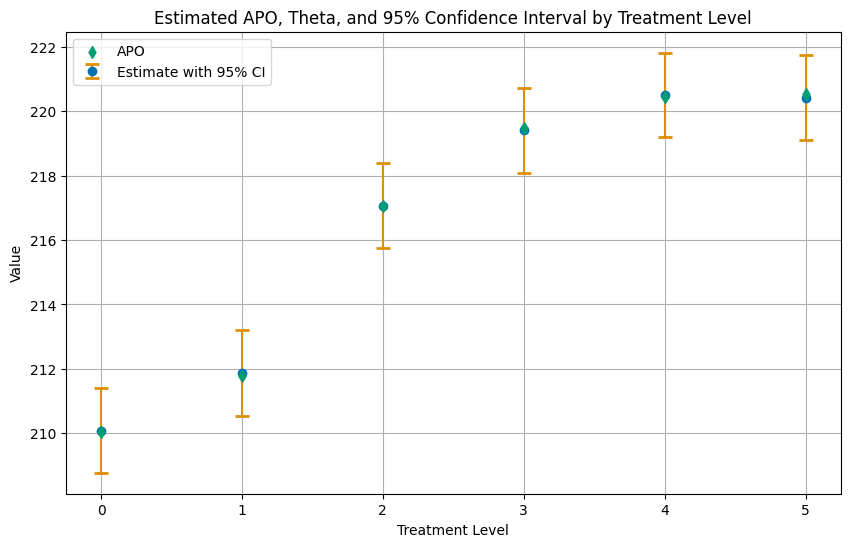

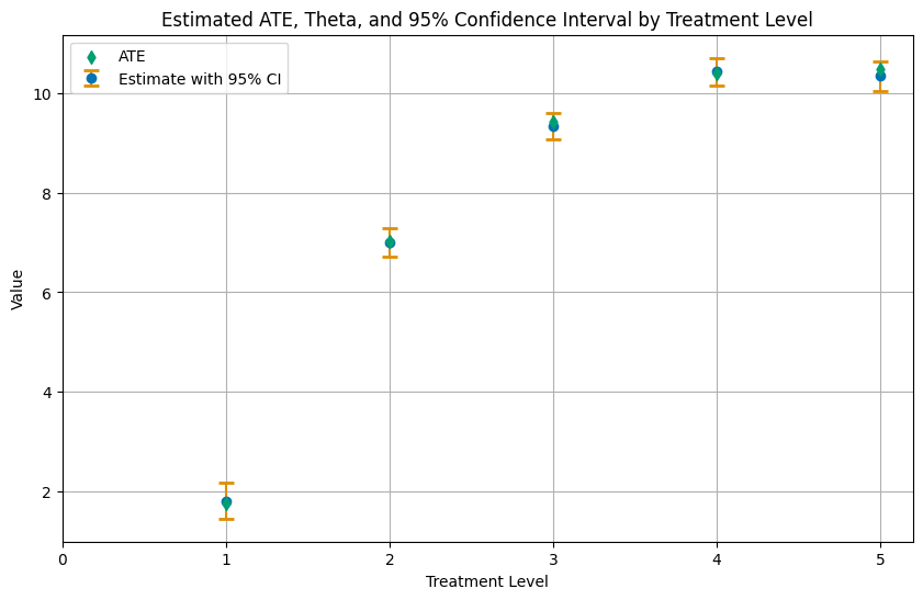
For a multi-valued or continuous treatment: estimate E[Y(d)] at each dose and the contrasts between them, all cross-fitted.
When treatment is endogenous, an instrument identifies the complier (LATE) effect via two-stage least squares — after you check the instrument is strong.
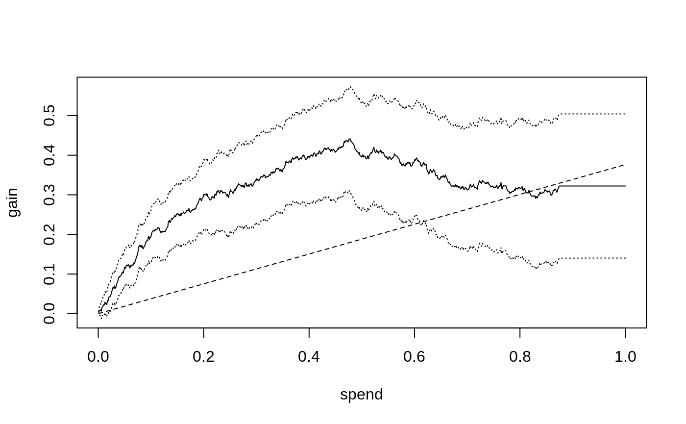
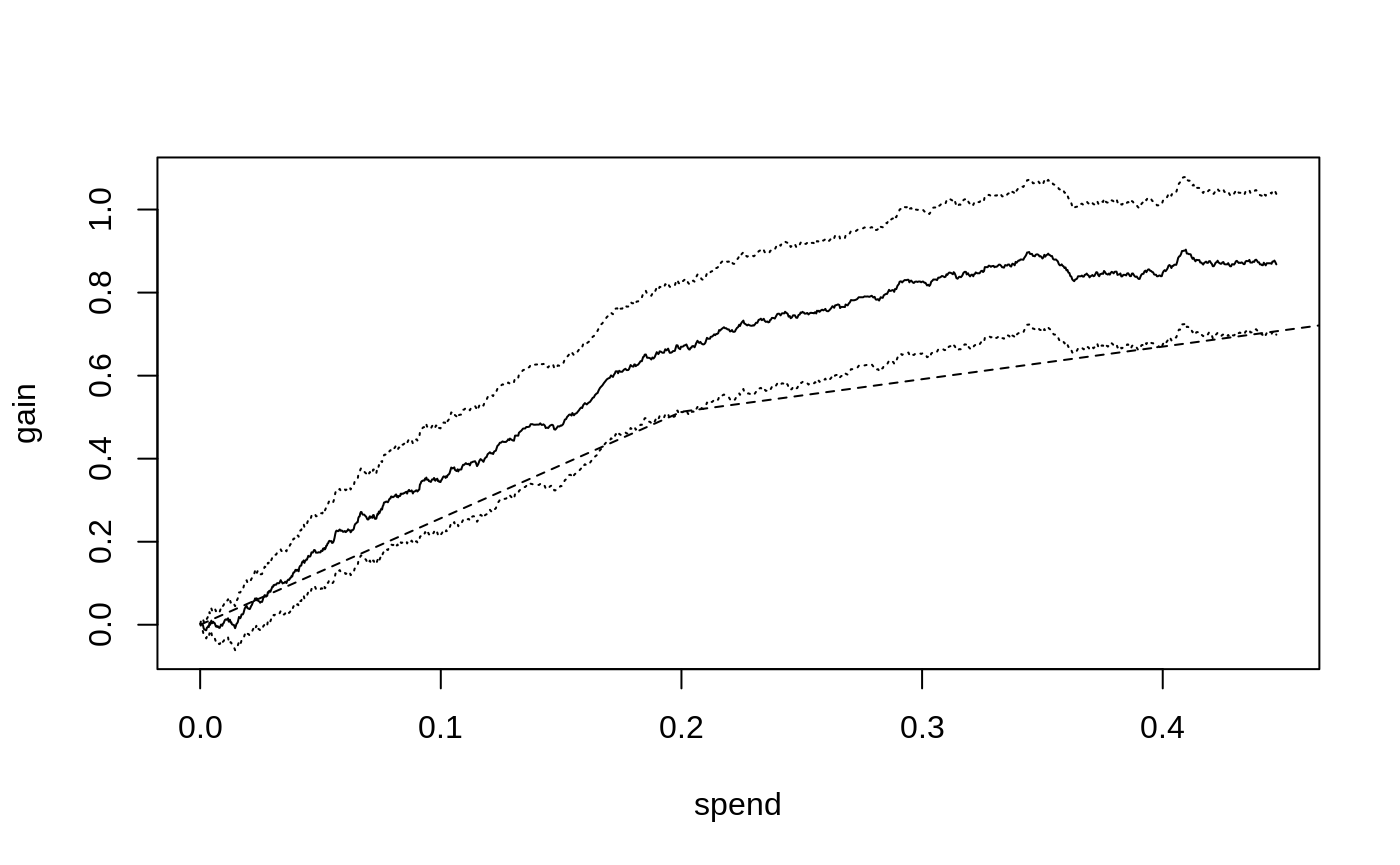
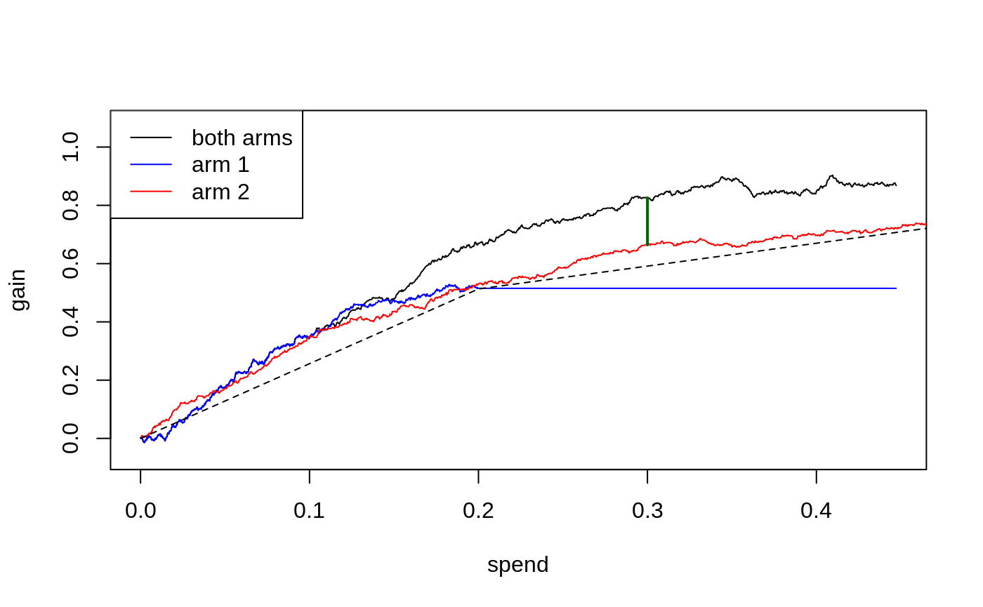
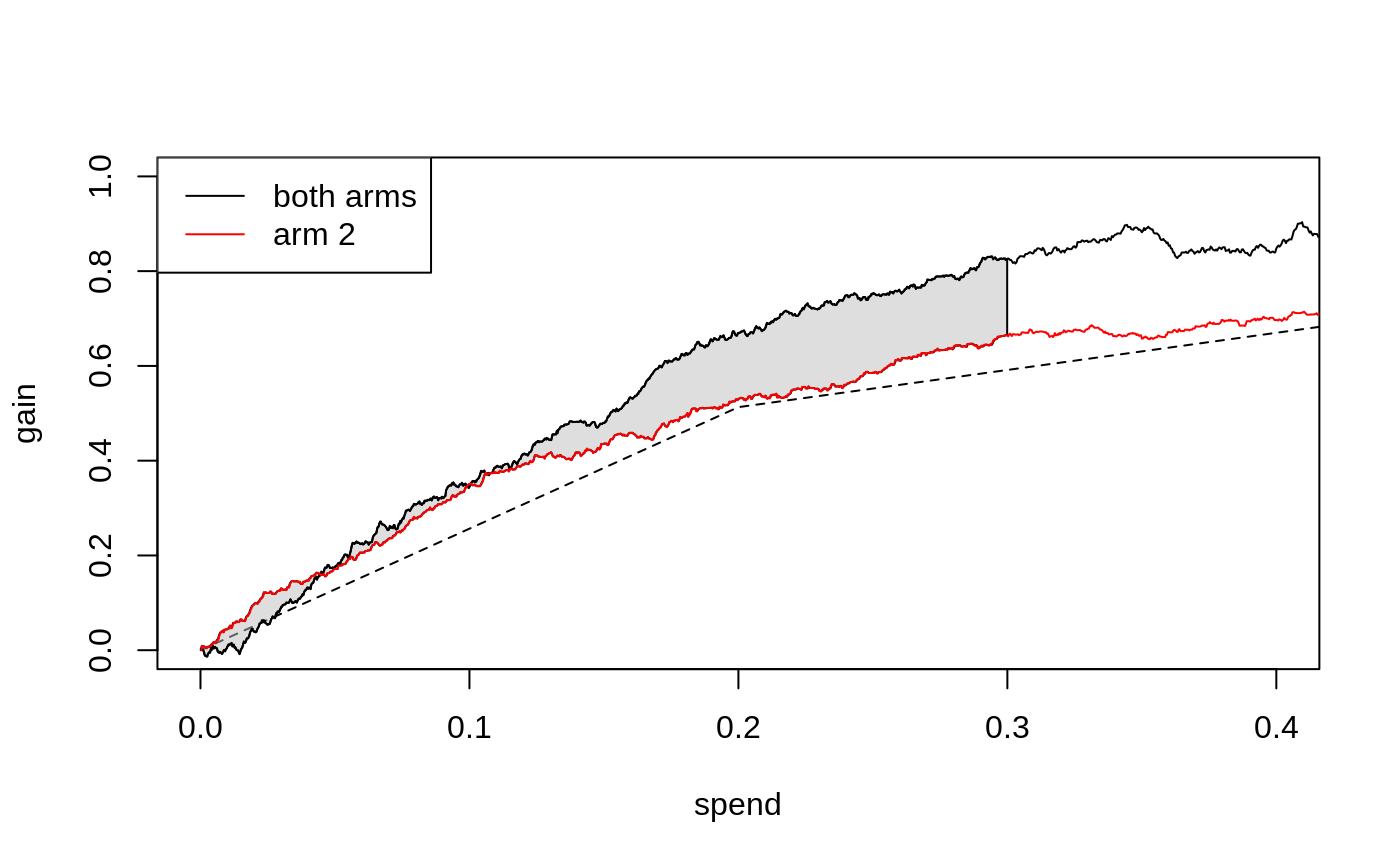
From CATEs to a budgeted treatment policy: causal forest → DR scores → cost matrix → maq Qini curve → pick the budget.
My side-by-side for staggered adoption: Callaway–Sant'Anna vs Gardner's two-stage vs Sun–Abraham — do the event studies agree?
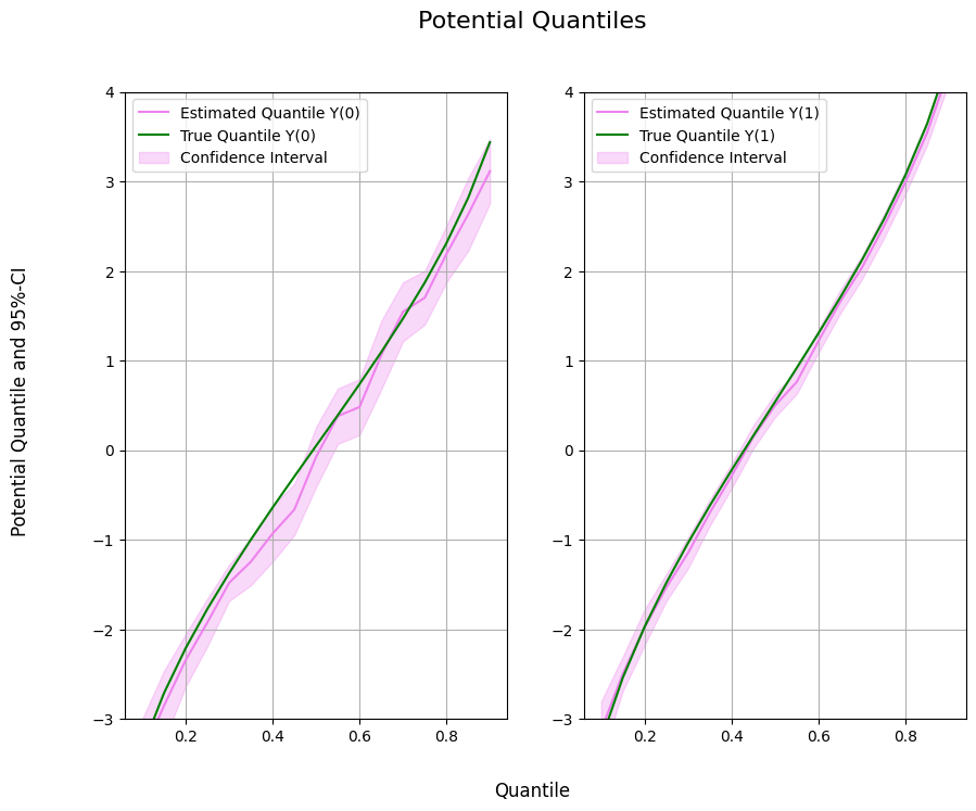
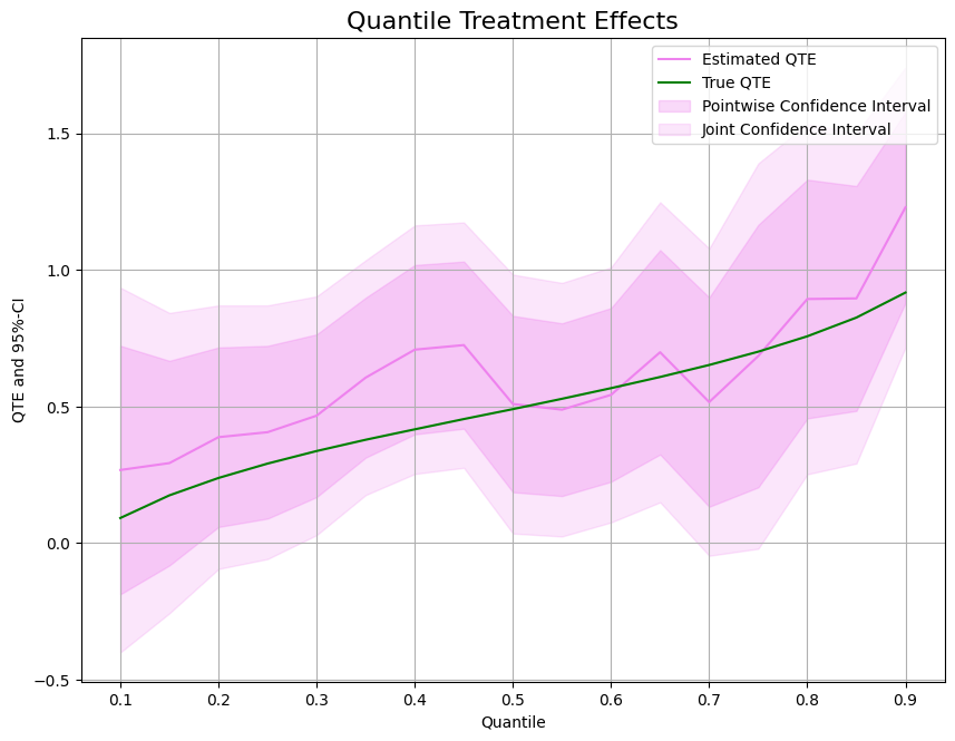
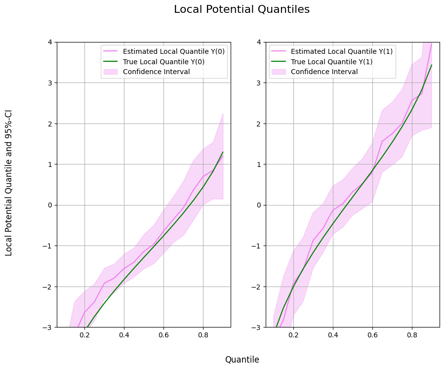
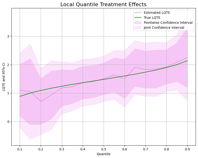
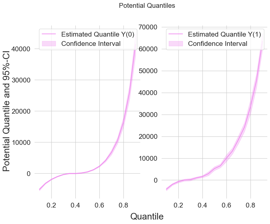
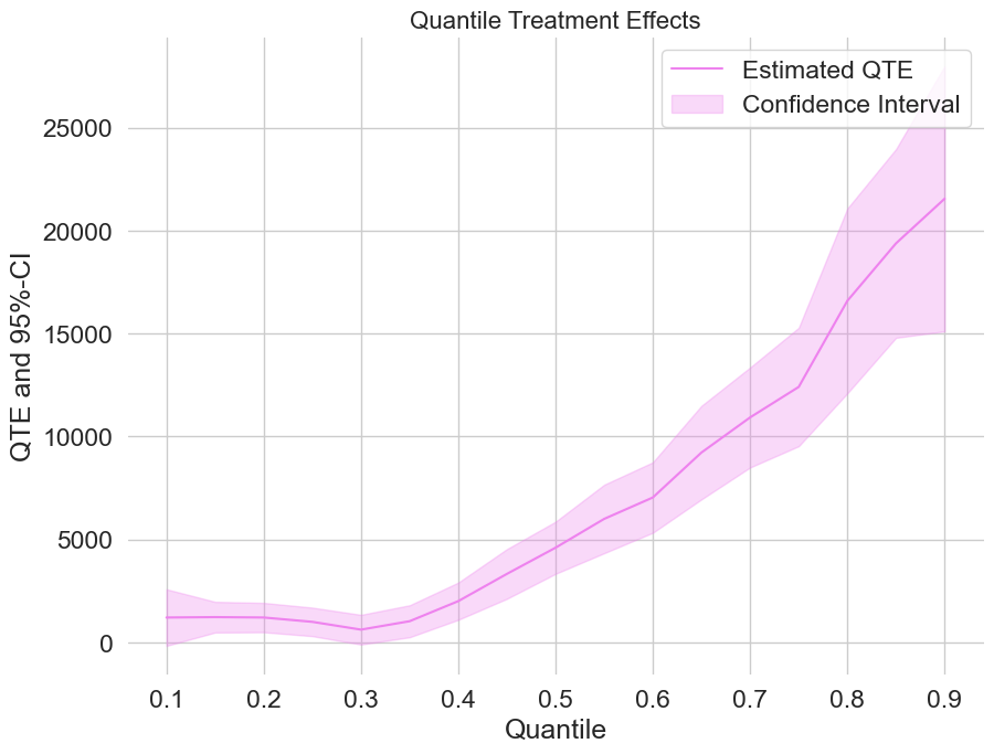
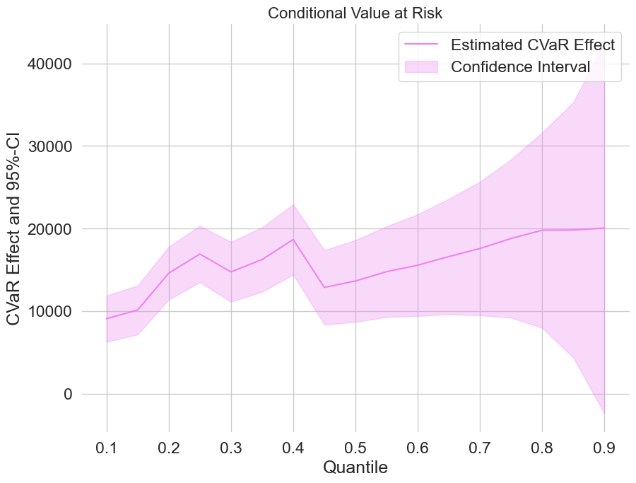
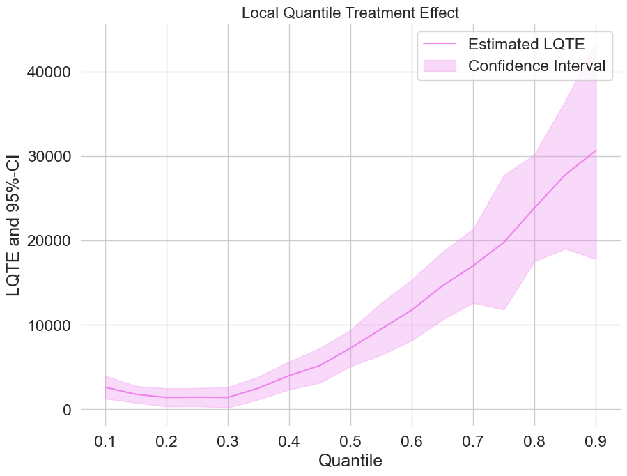
When the tails matter: estimate potential quantiles and the conditional value-at-risk of a treatment with Neyman-orthogonal scores.
My checklist for an observational effect: match, prove balance with cobalt, estimate on the matched sample, then quantify hidden-confounding risk with sensemakr.