@misc{grf,
  title        = {grf},
  author       = {Athey and Tibshirani and Wager},
  howpublished = {\url{https://grf-labs.github.io/grf/}},
  note         = {Software / documentation}
}Did the forest actually capture treatment-effect heterogeneity? Calibration → variable importance → BLP → omnibus tests.
Input · what goes in
A fitted causal forest (n=2000, p=10) you want to validate before trusting.
Show data format & exampleHide example
Format — one row per unit. A covariate matrix X (numeric), a binary treatment W ∈ {0,1}, and an outcome Y.
  X1     X2    X3    W    Y
 0.42  -1.1   0     1   3.10
-0.07   0.6   1     0   1.85
 1.20   0.3   0     1   4.02
Pipeline · the recipe ⑂ has parallel branches
↑ Click any step in the diagram to read its logic, code, assumptions & discussion.
[GRF] Causal forest
The core estimate — where the causal quantity itself is computed.
Fit with OOB predictions and variance.
Causal forest — Honest random forest for heterogeneous treatment effects — CATE for a binary treatment via GRF moment conditions.
cf <- causal_forest(X, Y, W)          # Y.hat, W.hat cross-fit
tau.hat <- predict(cf)$predictions    # OOB CATEs
- No comments on this step yet — be the first.
Log in to comment on this step.
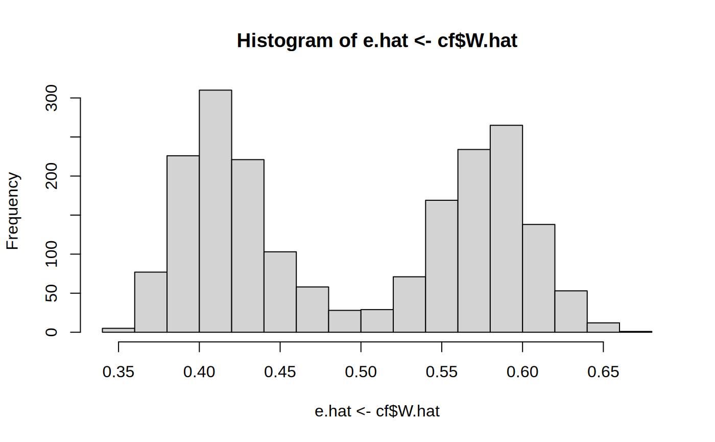
test_calibration()
A pre-flight check — run this before trusting any estimate downstream.
Mean-forest coefficient ≈ 1 says the average ATE is right; differential-forest coefficient ≈ 1 says heterogeneity is real.
test_calibration(cf) # mean & differential forest coefficients ≈ 1?
- No comments on this step yet — be the first.
Log in to comment on this step.
variable_importance()
A pre-flight check — run this before trusting any estimate downstream.
Which covariates the forest split on most often — sanity-check against domain knowledge.
variable_importance(cf)
- No comments on this step yet — be the first.
Log in to comment on this step.
best_linear_projection()
Heterogeneity — who is affected, and by how much, not just on average.
Linear projection of τ̂(x) on a hand-picked subset for human-readable heterogeneity.
best_linear_projection(cf, X[, c("age", "prior")])
- No comments on this step yet — be the first.
Log in to comment on this step.
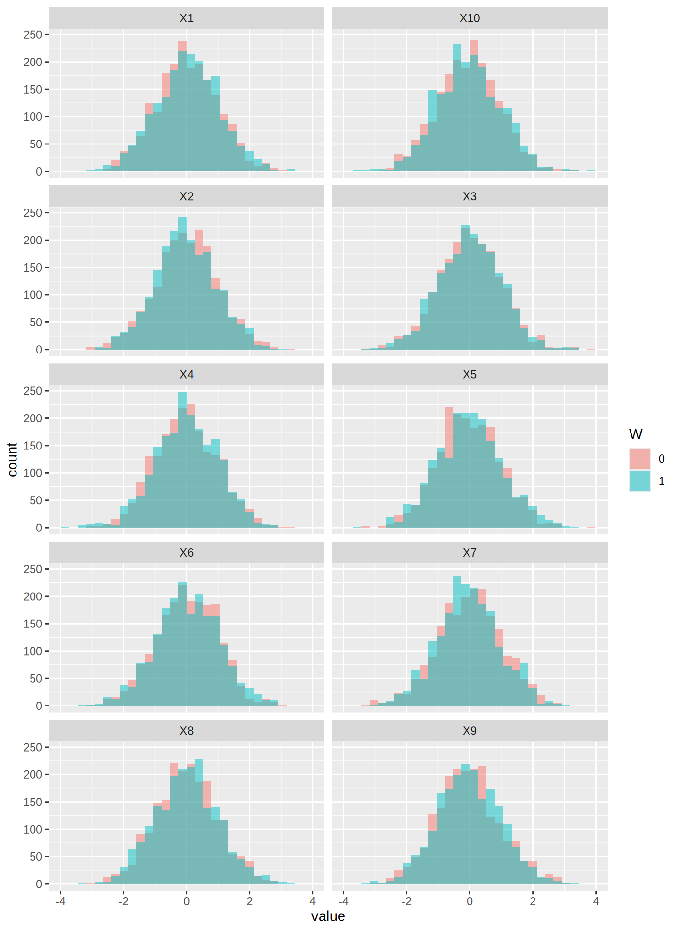
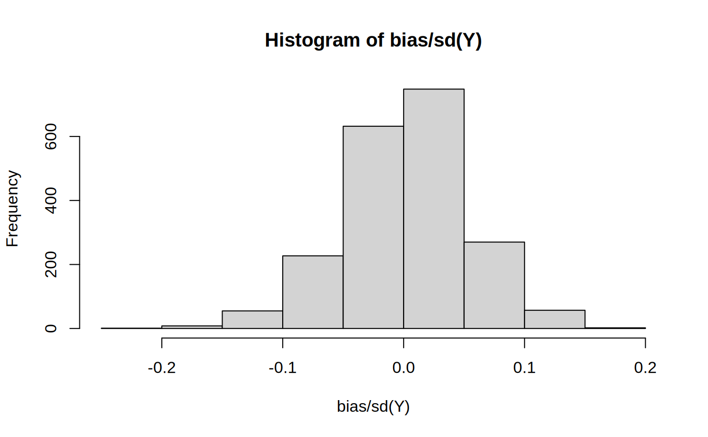
OOB residual checks
A pre-flight check — run this before trusting any estimate downstream.
Plot OOB CATEs against propensity & key covariates; large structure left here = under-fitting.
- No comments on this step yet — be the first.
Log in to comment on this step.
Fit-evaluation report
Reporting — turn the numbers into a figure or table a reader can act on.
Calibration table + importance bar chart + BLP table + residual scan, in one place.
- No comments on this step yet — be the first.
Log in to comment on this step.
Output · what you get 3 figures
Figures reproduced from grf — Athey, Tibshirani & Wager — unofficial community showcase; all credit to the original authors.
The GRF 'Evaluating a causal forest fit' tutorial. Before reading anything off a fitted forest, check that it's well-calibrated and that the heterogeneity isn't an artifact of noise. Then look at what's driving the splits and how the CATE relates to interpretable covariates. Unofficial summary.
Discussion (0)
Log in to join the discussion.