Workflow·4 steps·branched

Quantile treatment effects of 401(k) eligibility (DoubleML)

@doubleml ✓ P D · Jun 4, 2026 · 814 views

Source DoubleML — Bach, Chernozhukov, Kurz & Spindler

@misc{doubleml,
  title        = {DoubleML},
  author       = {Bach and Chernozhukov and Kurz and Spindler},
  howpublished = {\url{https://docs.doubleml.org/}},
  note         = {Software / documentation}
}

Summary by StatsDoge

Beyond the average: how 401(k) eligibility shifts net financial assets across the whole wealth distribution, estimated orthogonally.

Input · what goes in

Outcome Y (net assets), binary treatment D (eligibility), covariates X — the SIPP 401(k) sample.

Show data format & exampleHide example

Format — one row per household: net_tfa, e401 ∈ {0,1}, covariates X.

 net_tfa  e401  age  inc   educ
  12000     1    41  38k   13
   -400     0    53  21k   11

Pipeline · the recipe ⑂ has parallel branches

↑ Click any step in the diagram to read its logic, code, assumptions & discussion.

Data prep

Build DoubleMLData (net_tfa, e401, X)

Data preparation — shapes the raw inputs into what the estimator expects.

What happens here

Declare the outcome, the eligibility treatment, and covariates.

Reads from the input data Feeds into the final output

Key code

dml_data = dml.DoubleMLData(df, 'net_tfa', 'e401', x_cols=X)

Discussion on this step (0)

No comments on this step yet — be the first.

Estimation

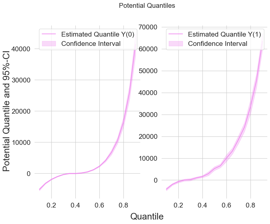
Estimate QTEs across the distribution

The core estimate — where the causal quantity itself is computed.

What happens here

A grid of quantiles, each a debiased potential-quantile contrast.

Formula

\mathrm{QTE}( au)=F^{-1}_{Y(1)}( au)-F^{-1}_{Y(0)}( au)

Reads from the input data Feeds into the final output

Key code

qte = dml.DoubleMLQTE(dml_data, ml_g, ml_m, quantiles=np.arange(.1,.95,.05)).fit()

Reference / docs ↗

Discussion on this step (0)

No comments on this step yet — be the first.

Inference

Simultaneous confidence bands

Uncertainty quantification — standard errors, intervals, and aggregation.

What happens here

Bootstrap joint bands so the whole QTE curve is covered at once.

Formula

F_{Y(d)}(y)=\mathbb{E}\!\left[\,\mathbb{1}\{Y(d)\le y\}\, ight]

Reads from the input data Feeds into the final output

Key code

qte.bootstrap(); qte.confint(joint=True)

Reference / docs ↗

Discussion on this step (0)

No comments on this step yet — be the first.

Reporting

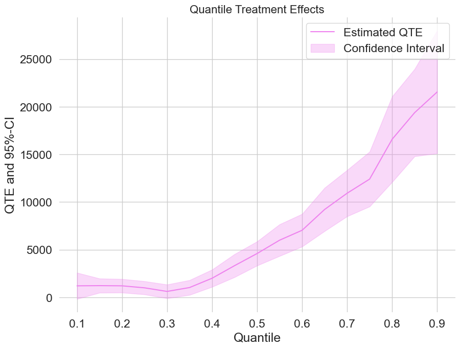
Plot the QTE curve

Reporting — turn the numbers into a figure or table a reader can act on.

What happens here

Effect against quantile τ — where in the distribution the policy bites.

Reads from the input data Feeds into the final output

Key code

# QTE vs quantile, with joint bands

Discussion on this step (0)

No comments on this step yet — be the first.

Output · what you get 4 figures

Fig 1Quantile treatment effects across the distribution of net financial assets.

Fig 2QTE point estimates with pointwise confidence intervals at each quantile.

Fig 3QTE with simultaneous (joint) confidence bands across quantiles.

Fig 4Comparison of QTE estimates across model/learner choices.

Figures reproduced from DoubleML — Bach, Chernozhukov, Kurz & Spindler — unofficial community showcase; all credit to the original authors.

⚠️ Unofficial community showcase of a DoubleML example. Not affiliated with the authors; figures are from the public documentation. All credit to Bach, Chernozhukov, Kurz & Spindler.

Beyond the average: how 401(k) eligibility shifts net financial assets across the whole wealth distribution, estimated orthogonally.

Quantile treatment effects of 401(k) eligibility (DoubleML)

Input · what goes in

Pipeline · the recipe ⑂ has parallel branches

Output · what you get 4 figures

Discussion (0)