@misc{grf,
  title        = {grf},
  author       = {Athey and Tibshirani and Wager},
  howpublished = {\url{https://grf-labs.github.io/grf/}},
  note         = {Software / documentation}
}Causal forest → train/eval split → RATE with both AUTOC and Qini → TOC plot.
Input · what goes in
A fitted causal forest plus a held-out evaluation sample (X, W, Y).
Show data format & exampleHide example
Format — one row per unit. A covariate matrix X (numeric), a binary treatment W ∈ {0,1}, and an outcome Y.
  X1     X2    X3    W    Y
 0.42  -1.1   0     1   3.10
-0.07   0.6   1     0   1.85
 1.20   0.3   0     1   4.02
Pipeline · the recipe ⑂ has parallel branches
↑ Click any step in the diagram to read its logic, code, assumptions & discussion.
[GRF] Regression forest
Data preparation — shapes the raw inputs into what the estimator expects.
Cross-fit nuisances.
Regression forest — Honest non-parametric regression for E[Y|X], with out-of-bag predictions and pointwise CIs.
rf <- regression_forest(X, Y)
Y.hat <- predict(rf)$predictions
- No comments on this step yet — be the first.
Log in to comment on this step.
[GRF] Causal forest
The core estimate — where the causal quantity itself is computed.
Causal forest on the training half; produce CATE priorities.
Causal forest — Honest random forest for heterogeneous treatment effects — CATE for a binary treatment via GRF moment conditions.
cf <- causal_forest(X, Y, W)          # Y.hat, W.hat cross-fit
tau.hat <- predict(cf)$predictions    # OOB CATEs
- No comments on this step yet — be the first.
Log in to comment on this step.
Train / evaluation split
Data preparation — shapes the raw inputs into what the estimator expects.
Hold out an independent half to fit the evaluation forest — RATE needs out-of-sample priorities.
idx <- sample(n, n / 2)            # independent train / eval split
train <- data[idx, ]; eval <- data[-idx, ]
- No comments on this step yet — be the first.
Log in to comment on this step.
[GRF] Rank-weighted ATE — RATE / AUTOC / Qini
Heterogeneity — who is affected, and by how much, not just on average.
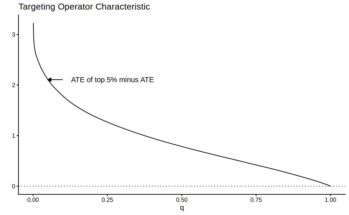
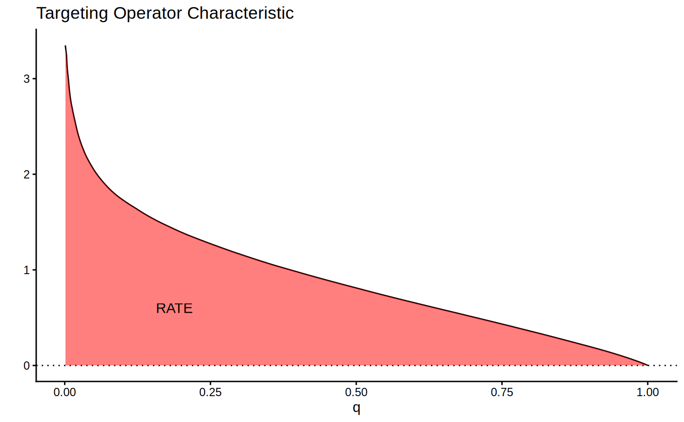
AUTOC: area under the TOC, sensitive to concentrated benefit.
Rank-weighted ATE — RATE / AUTOC / Qini — Evaluate how well a CATE estimate prioritizes treatment: TOC curve, AUTOC and Qini with confidence intervals.
rate <- rank_average_treatment_effect(eval.forest, priorities = tau.hat)
plot(rate)                          # TOC curve
rate$estimate / rate$std.err        # AUTOC z-stat
- No comments on this step yet — be the first.
Log in to comment on this step.
[GRF] Rank-weighted ATE — RATE / AUTOC / Qini
Heterogeneity — who is affected, and by how much, not just on average.
Qini: weights by treated fraction, sensitive to broad benefit.
Rank-weighted ATE — RATE / AUTOC / Qini — Evaluate how well a CATE estimate prioritizes treatment: TOC curve, AUTOC and Qini with confidence intervals.
rate <- rank_average_treatment_effect(eval.forest, priorities = tau.hat)
plot(rate)                          # TOC curve
rate$estimate / rate$std.err        # AUTOC z-stat
- No comments on this step yet — be the first.
Log in to comment on this step.
TOC plot + AUTOC/Qini table
Reporting — turn the numbers into a figure or table a reader can act on.
Plot the TOC with CIs; report both summaries and whether each clears zero.
- No comments on this step yet — be the first.
Log in to comment on this step.
Output · what you get 4 figures
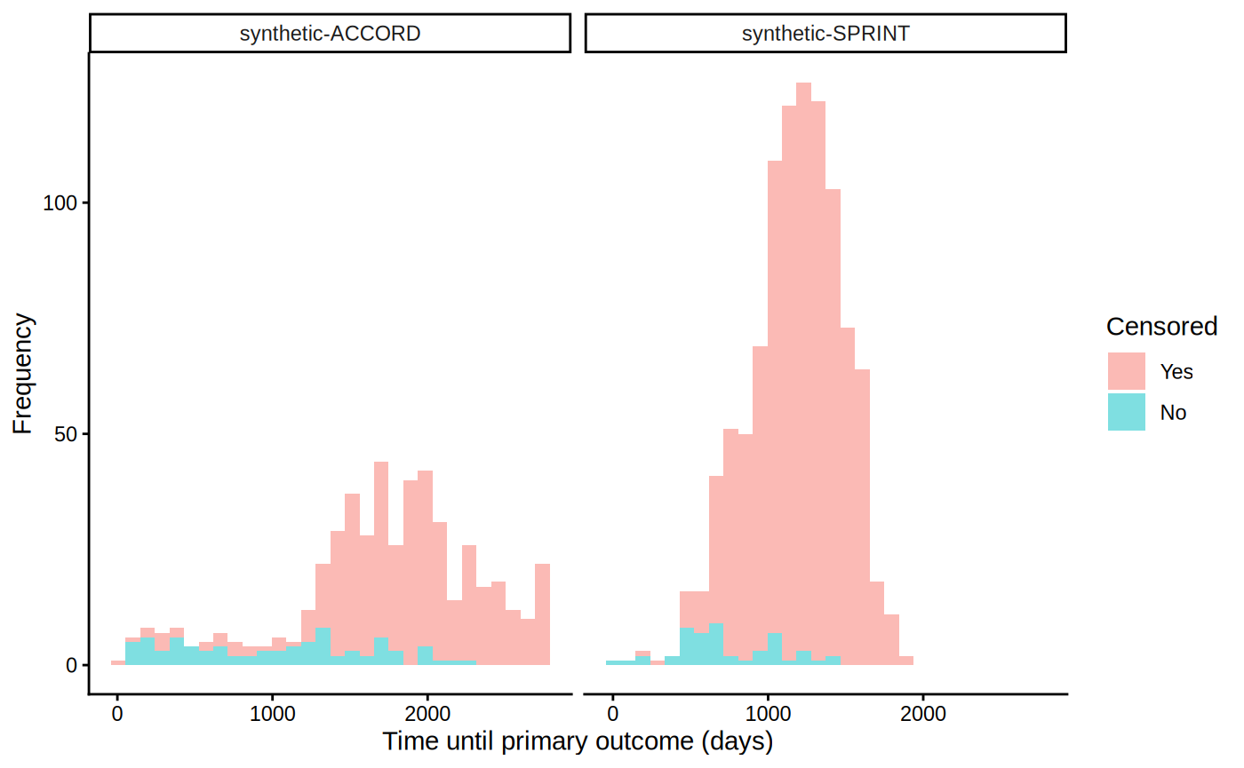
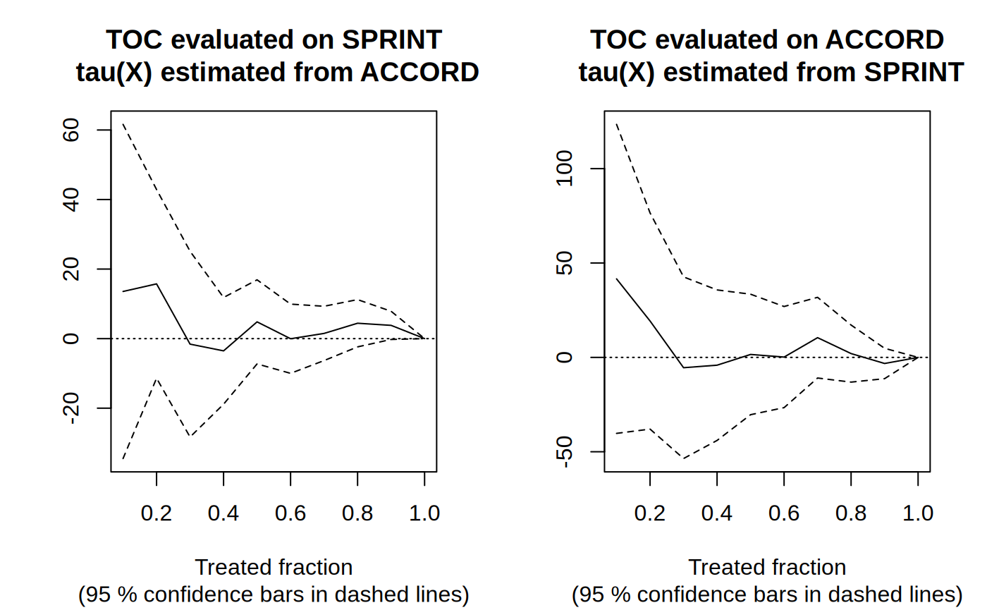
Figures reproduced from grf — Athey, Tibshirani & Wager — unofficial community showcase; all credit to the original authors.
The GRF 'Assessing heterogeneity with RATE' tutorial. Fit on one half, evaluate prioritization on the other; report AUTOC (rewards concentrated heterogeneity) and Qini (rewards broad effects) with CIs. Unofficial summary.
Discussion (2)
Log in to join the discussion.
Running both AUTOC and Qini side by side is the right move — they answer different targeting questions and disagreeing is informative.
Yep. If AUTOC fires but Qini doesn't, your benefit is concentrated in a small group.
The independent train/eval split is non-negotiable here. Priorities have to be out-of-sample or RATE is optimistic.