@misc{grf,
  title        = {grf},
  author       = {Athey and Tibshirani and Wager},
  howpublished = {\url{https://grf-labs.github.io/grf/}},
  note         = {Software / documentation}
}Censoring check → causal survival forest → RMST-scale AIPW ATE → calibration → report.
Input · what goes in
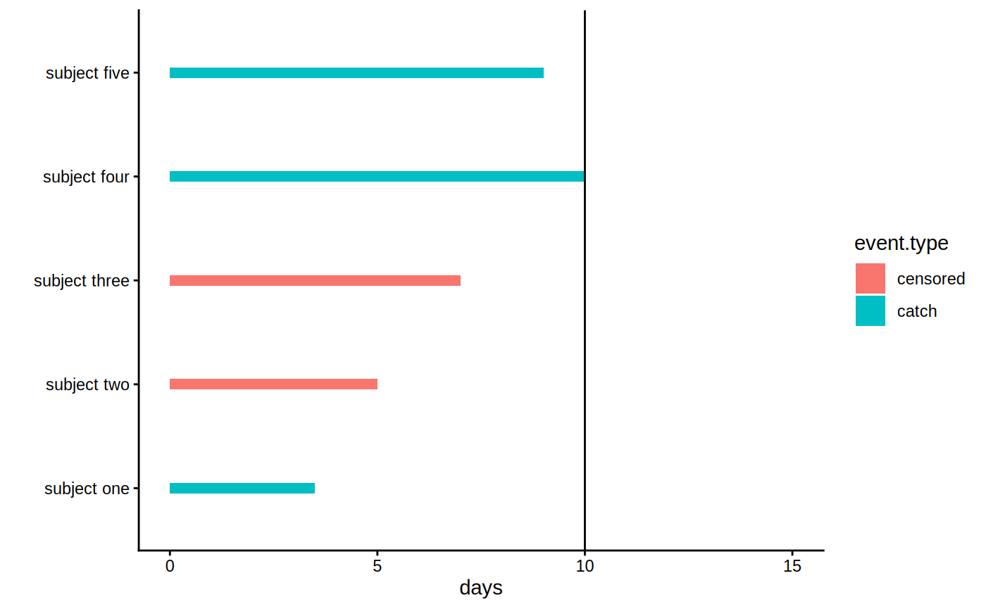
Right-censored survival time Y, event indicator D, treatment W, covariates X.
Show data format & exampleHide example
Format — one row per unit. Covariates X, binary treatment W, a (possibly censored) time Y, and an event indicator D (1 = event, 0 = censored).
  X1    X2   W     Y     D
 0.4  -1.1  1   12.3   1
-0.1   0.6  0   30.0   0   # censored
 1.2   0.3  1    8.7   1
Pipeline · the recipe ⑂ has parallel branches
↑ Click any step in the diagram to read its logic, code, assumptions & discussion.
[GRF] Survival forest
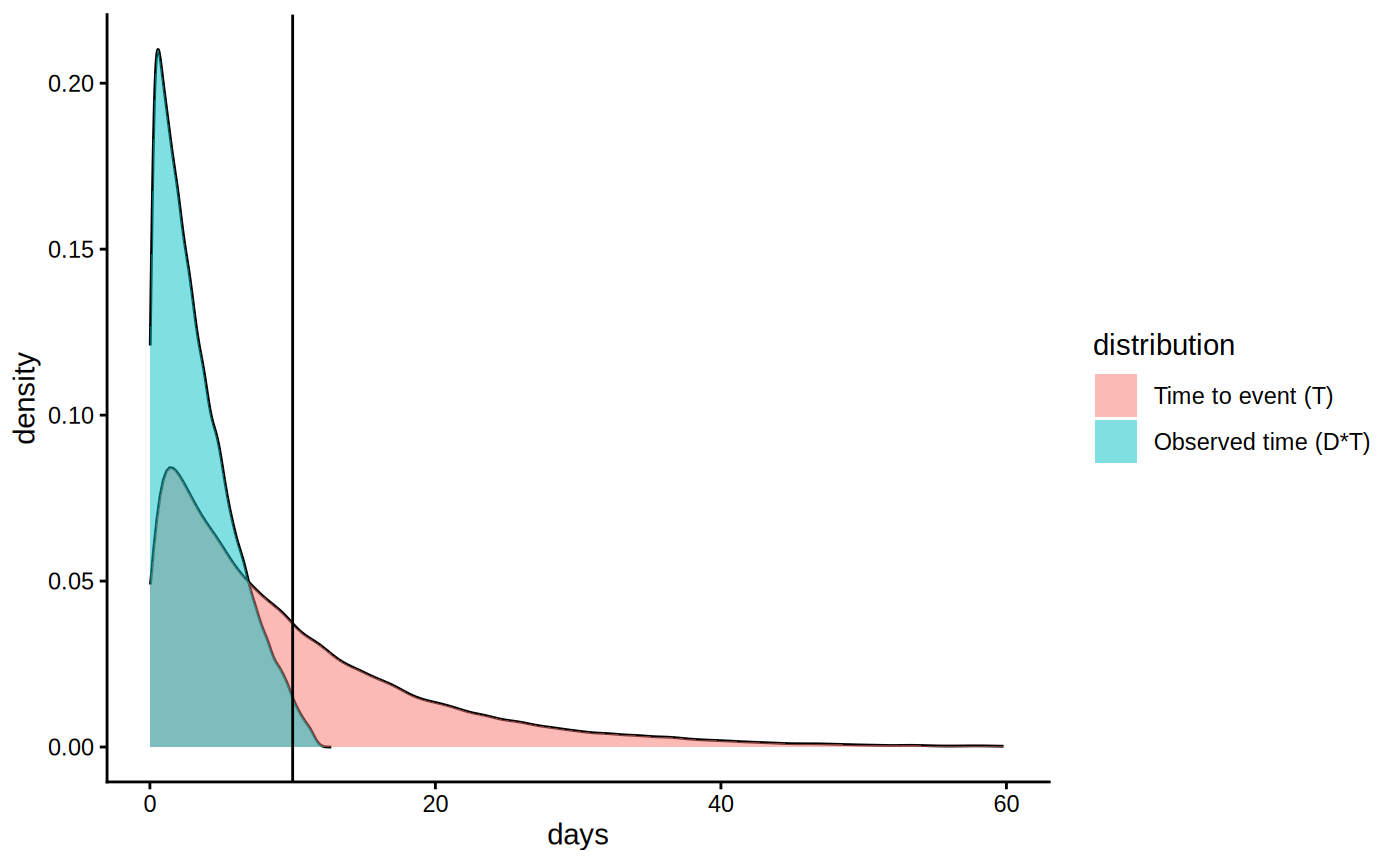
A pre-flight check — run this before trusting any estimate downstream.
Inspect the conditional censoring/survival curves; pick a horizon h with enough events.
Survival forest — Non-parametric conditional survival function S(t | X) under right-censoring.
sf <- survival_forest(X, Y, D)
predict(sf)$predictions             # conditional survival curve
- No comments on this step yet — be the first.
Log in to comment on this step.
[GRF] Causal survival forest
The core estimate — where the causal quantity itself is computed.
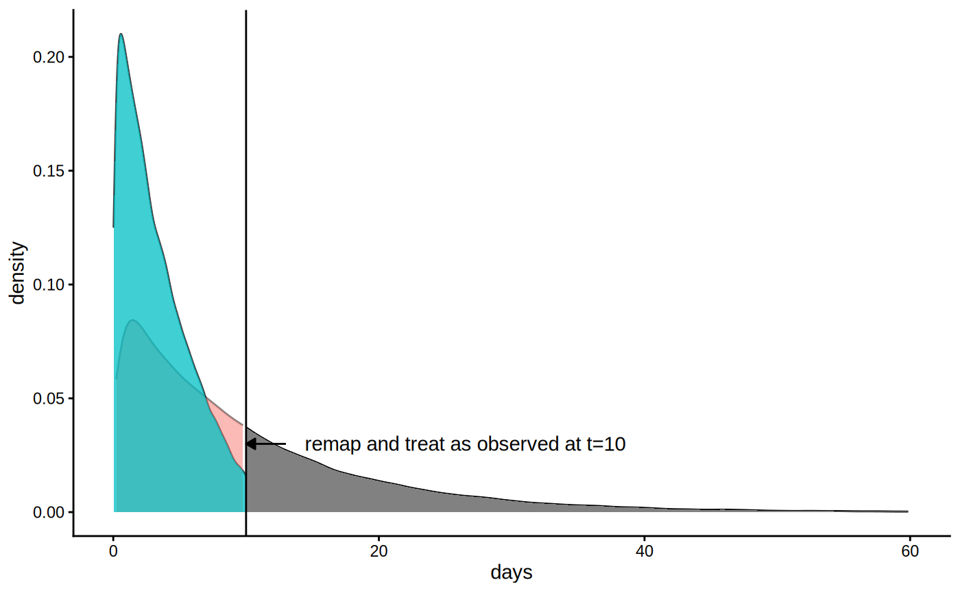
Estimate τ(x) as the difference in restricted mean survival time up to h.
Causal survival forest — CATE with right-censored, time-to-event outcomes (RMST or survival probability).
csf <- causal_survival_forest(X, Y, W, D, horizon = h)
predict(csf)$predictions            # CATE on the RMST scale
- No comments on this step yet — be the first.
Log in to comment on this step.
[GRF] AIPW average treatment effect
Uncertainty quantification — standard errors, intervals, and aggregation.
Aggregate to a doubly-robust RMST-difference ATE.
AIPW average treatment effect — Doubly-robust ATE / ATT / ATC / overlap-weighted effect from a trained causal forest, via augmented IPW.
average_treatment_effect(cf, target.sample = "all")      # ATE
average_treatment_effect(cf, target.sample = "treated")  # ATT
- No comments on this step yet — be the first.
Log in to comment on this step.
test_calibration()
A pre-flight check — run this before trusting any estimate downstream.
Check the forest is calibrated on the RMST scale.
test_calibration(cf) # mean & differential forest coefficients ≈ 1?
- No comments on this step yet — be the first.
Log in to comment on this step.
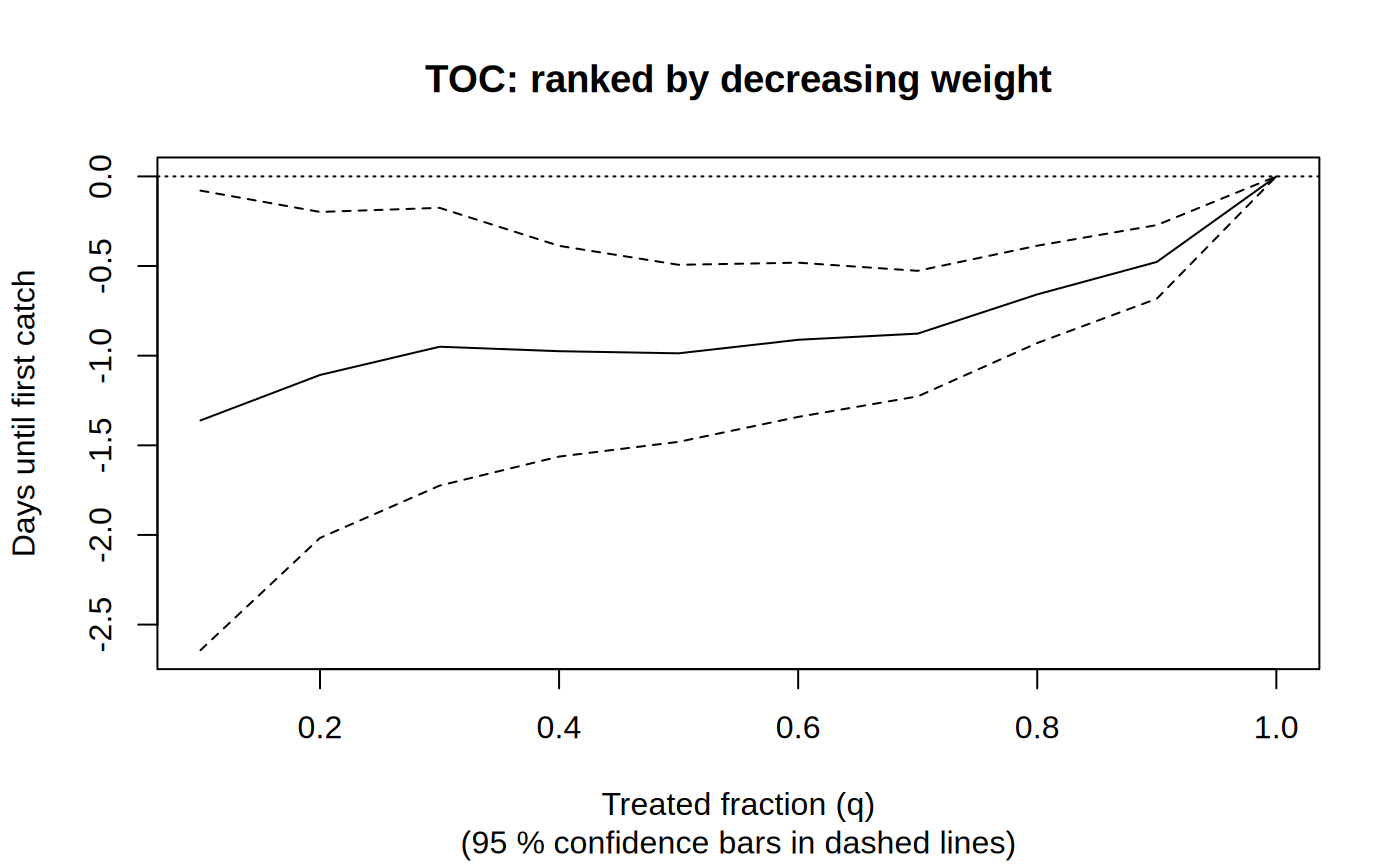
RMST difference by subgroup
Reporting — turn the numbers into a figure or table a reader can act on.
Report the survival benefit overall and for key subgroups, with the censoring caveat.
- No comments on this step yet — be the first.
Log in to comment on this step.
Output · what you get 4 figures
Figures reproduced from grf — Athey, Tibshirani & Wager — unofficial community showcase; all credit to the original authors.
The GRF survival tutorial. Model censoring first, estimate CATE on the RMST scale, then aggregate and validate. Unofficial summary.
Discussion (2)
Log in to join the discussion.
Modelling censoring as step 1 instead of an afterthought is exactly right. So many survival analyses get this backwards.
The horizon-sensitivity caveat in the report step is a nice touch. RMST is horizon-dependent and people forget.