@misc{cobalt,
  title        = {cobalt},
  author       = {Noah Greifer},
  howpublished = {\url{https://ngreifer.github.io/cobalt/}},
  note         = {Software / documentation}
}Before you trust an observational estimate, prove balance: SMDs, overlap, and a Love plot before vs after adjustment.
Input · what goes in
A binary treatment and the covariates you'll adjust for (e.g. the Lalonde job-training data).
Show data format & exampleHide example
Format — one row per unit: treatment W ∈ {0,1} and covariates X.
  W   age  educ   race   re74    re75
  1    37    11   black     0       0
  0    30    12   white  4100    3800
Pipeline · the recipe
↑ Click any step in the diagram to read its logic, code, assumptions & discussion.
Treatment W + covariates X
Data preparation — shapes the raw inputs into what the estimator expects.
Binary treatment plus the covariates to balance (Lalonde: age, educ, race, re74, re75).
data("lalonde", package = "cobalt")
- No comments on this step yet — be the first.
Log in to comment on this step.
Estimate weights / matches (WeightIt / MatchIt)
Data preparation — shapes the raw inputs into what the estimator expects.
Fit a propensity model; produce IPW weights or matched sets.
library(WeightIt)
w <- weightit(treat ~ age + educ + race + re74 + re75, lalonde, estimand = "ATT")
- No comments on this step yet — be the first.
Log in to comment on this step.
[cobalt] Balance tables & Love plots — bal.tab()
A pre-flight check — run this before trusting any estimate downstream.
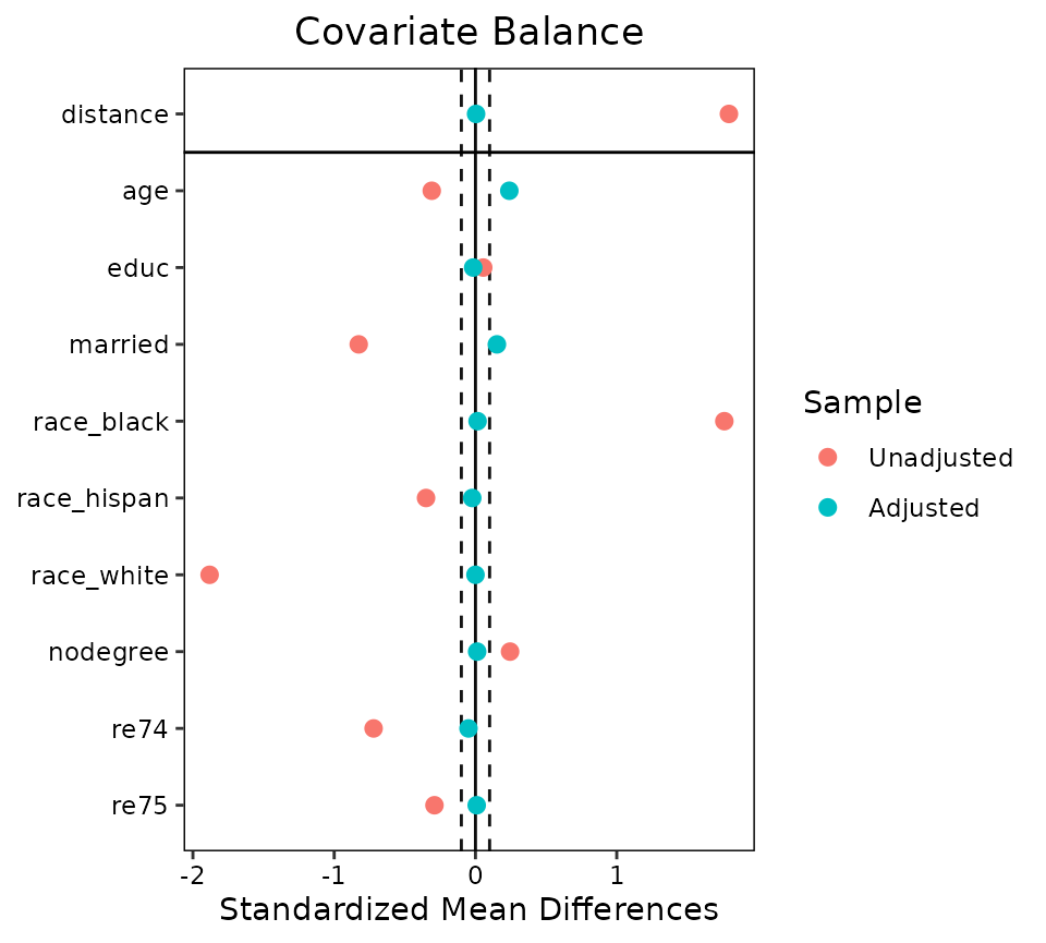
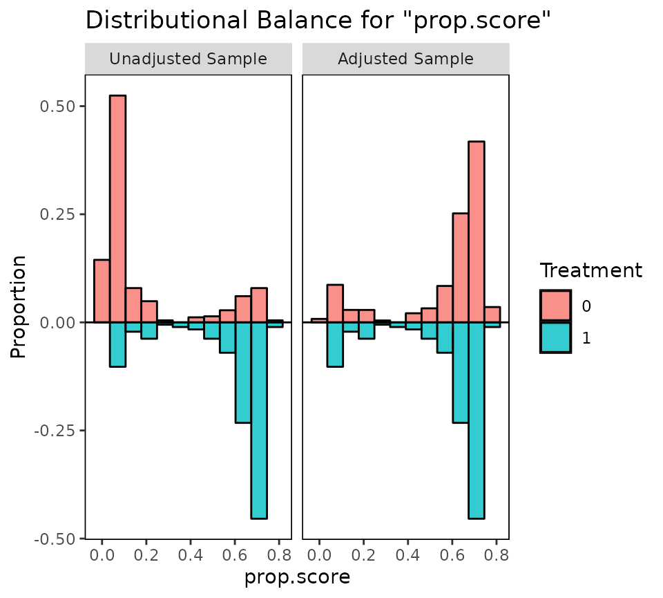
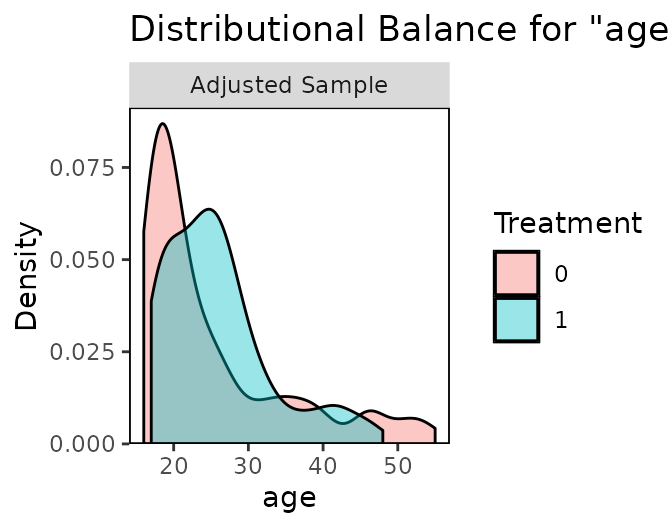
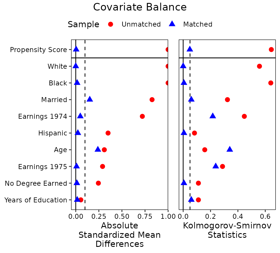
bal.tab(): standardized mean differences, adjusted vs unadjusted.
Balance tables & Love plots — bal.tab() — Assess covariate balance before/after matching or weighting: standardized mean differences, KS stats, and the publication-ready Love plot.
bal.tab(w, un = TRUE)
- No comments on this step yet — be the first.
Log in to comment on this step.
love.plot()
Reporting — turn the numbers into a figure or table a reader can act on.
Love plot of |SMD| with the 0.1 balance threshold; show before vs after.
love.plot(w, thresholds = c(m = 0.1))
- No comments on this step yet — be the first.
Log in to comment on this step.
Output · what you get 4 figures
Figures reproduced from cobalt — Noah Greifer — unofficial community showcase; all credit to the original authors.
From the cobalt vignette (Lalonde). Estimate weights/matches, then check that adjustment actually balanced the covariates. Unofficial summary.
Discussion (2)
Log in to join the discussion.
A causal estimate from observational data without a Love plot is a vibe, not evidence. cobalt makes the balance check trivial.
100%. I put love.plot() in every appendix now. Reviewers love it.
Works with MatchIt, WeightIt, raw weights… one balance API for everything. Underrated.