@misc{honestdid,
  title        = {HonestDiD},
  author       = {Rambachan and Roth},
  howpublished = {\url{https://github.com/asheshrambachan/HonestDiD}},
  note         = {Software / documentation}
}Stop betting everything on a pre-trends test. Bound how far the post-treatment trend can deviate (relative-magnitudes / smoothness classes), then report the union of confidence intervals over that class plus the breakdown M̄* — the trend size that just nulls the effect.
Input · what goes in
An event-study: the vector of pre- and post-treatment coefficients and their covariance matrix (from any DiD / event-study estimator).
Show data format & exampleHide example
Format — the event-study coefficient vector betahat and its covariance sigma (e.g. from fixest/did).
library(HonestDiD)
# betahat: pre + post event-time coefficients
# sigma:   their covariance matrix; numPrePeriods / numPostPeriods
Pipeline · the recipe ⑂ has parallel branches
↑ Click any step in the diagram to read its logic, code, assumptions & discussion.
Start from event-study coefficients
Data preparation — shapes the raw inputs into what the estimator expects.
Take β̂ (pre- and post-treatment event-time coefficients) and its covariance Σ from whatever DiD estimator you trust.
es <- fixest::feols(y ~ i(rel_time, ref = -1) | id + period, df)
betahat <- coef(es); sigma <- vcov(es)
- No comments on this step yet — be the first.
Log in to comment on this step.
Read the pre-trends, don't just test them
A pre-flight check — run this before trusting any estimate downstream.
A failed pre-trends test is low-power and a passed one isn't a green light. Treat the post-period bias δ as something to bound, not assume away.
# post-period coefficient = causal effect + differential trend
- No comments on this step yet — be the first.
Log in to comment on this step.
Bound the deviation: relative magnitudes / smoothness
A robustness check — does the headline result survive a different lens?
Restrict δ to a transparent class — no bigger than M̄× the largest pre-period wiggle (relative magnitudes), or boundedly nonlinear (smoothness).
delta_rm <- createSensitivityResults_relativeMagnitudes(
    betahat, sigma, numPrePeriods, numPostPeriods, Mbarvec = c(0.5,1,1.5,2))
- No comments on this step yet — be the first.
Log in to comment on this step.
Robust confidence set & breakdown value
Uncertainty quantification — standard errors, intervals, and aggregation.
Report the union of confidence intervals over the allowed δ, and the breakdown M̄* — how much trend the conclusion can survive.
robust <- createSensitivityResults_relativeMagnitudes(...)
createSensitivityPlot_relativeMagnitudes(robust, originalResults)
- No comments on this step yet — be the first.
Log in to comment on this step.
Output · what you get 2 figures
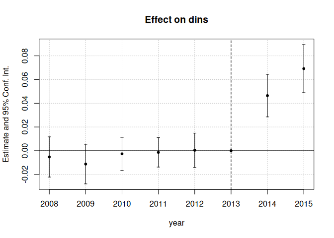
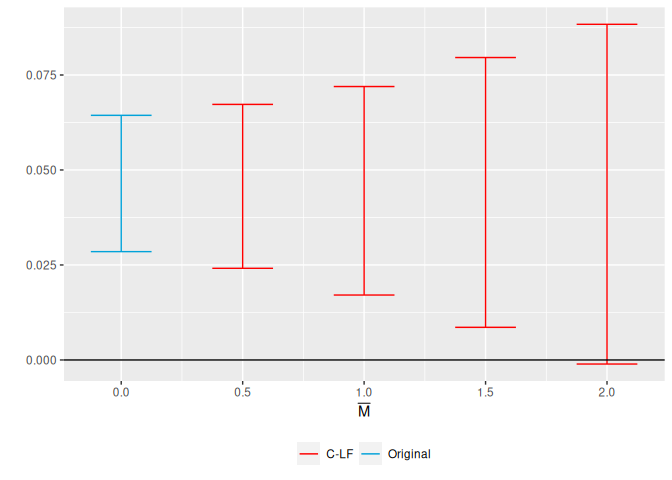
Figures reproduced from HonestDiD — Rambachan & Roth — unofficial community showcase; all credit to the original authors.
⚠️ Unofficial community showcase of honestdid. Not affiliated with the authors; all credit to them.
Stop betting everything on a pre-trends test. Allow the post-treatment trend to deviate within a transparent class, and report the confidence set — and the breakdown value where the effect would vanish.
Discussion (2)
Log in to join the discussion.
Replacing the pre-trends test with explicit bounds is the right move. The breakdown M̄* is exactly what referees keep asking me for.
I report the relative-magnitudes set next to the point estimate by default now — it pre-empts the 'but parallel trends' question.
Same. Pairing it with the event-study plot makes the whole argument legible in one figure.