@misc{dowhy,
  title        = {DoWhy},
  author       = {Sharma and Kiciman and others},
  howpublished = {\url{https://www.pywhy.org/dowhy/}},
  note         = {Software / documentation}
}A causal-graph–first recipe: write down the DAG, let the algorithm read off the backdoor adjustment set, plug any estimator in, and end with refutation tests (placebo treatment, random common cause) that try to falsify your effect. The discipline is in step 4.
Input · what goes in
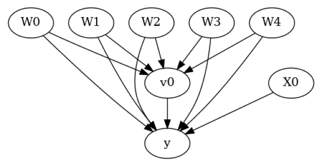
A dataset plus a causal graph (DAG) naming treatment, outcome, confounders and any instruments — the assumptions you're willing to defend.
Show data format & exampleHide example
Format — a tidy table together with a causal graph (DOT/GML) over treatment v0, outcome y and confounders W*.
import dowhy.datasets
d = dowhy.datasets.linear_dataset(
        beta=10, num_common_causes=5, num_instruments=1, num_samples=1000)
# d['df']: v0 (treatment), y (outcome), W0..W4 (confounders), X0
Pipeline · the recipe ⑂ has parallel branches
↑ Click any step in the diagram to read its logic, code, assumptions & discussion.
Model — encode the causal graph
Data preparation — shapes the raw inputs into what the estimator expects.
State the DAG over treatment, outcome, confounders and instruments. The assumptions go in up front, as a graph, not buried in a regression.
from dowhy import CausalModel
model = CausalModel(data=df, treatment='v0', outcome='y', graph=gml_graph)
- No comments on this step yet — be the first.
Log in to comment on this step.
Identify — apply the backdoor criterion
A pre-flight check — run this before trusting any estimate downstream.
DoWhy searches the graph for a valid adjustment set (backdoor), or an instrument/front-door, and returns the estimand symbolically — before touching the data.
estimand = model.identify_effect(proceed_when_unidentifiable=False)
- No comments on this step yet — be the first.
Log in to comment on this step.
Estimate — adjust for the backdoor set
The core estimate — where the causal quantity itself is computed.
Plug in any estimator for the identified estimand: linear adjustment, propensity weighting/matching, or a DML/forest backend.
est = model.estimate_effect(estimand,
        method_name='backdoor.propensity_score_weighting')
- No comments on this step yet — be the first.
Log in to comment on this step.
Refute — placebo & unobserved-confounder tests
A robustness check — does the headline result survive a different lens?
The step that earns trust: a random common cause shouldn't change τ̂; a placebo (permuted) treatment should drive it to zero; subsetting shouldn't move it much.
model.refute_estimate(estimand, est,
        method_name='placebo_treatment_refuter')
- No comments on this step yet — be the first.
Log in to comment on this step.
Output · what you get 2 figures
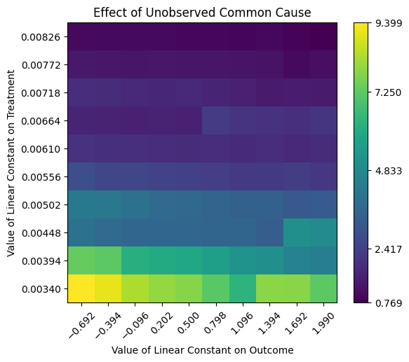
Figures reproduced from DoWhy — PyWhy / Microsoft (Sharma, Kiciman et al.) — unofficial community showcase; all credit to the original authors.
⚠️ Unofficial community showcase of dowhy. Not affiliated with the authors; all credit to them.
Make your assumptions explicit: draw a causal graph, identify the estimand by the backdoor criterion, estimate it, then actively try to refute it with placebo and confounding tests.
Discussion (2)
Log in to join the discussion.
The refute step is what sells DoWhy to me — placebo and random-common-cause as a default habit, not an afterthought.
Encoding the DAG up front forces the awkward assumptions into the open. Wish more pipelines did this.
Exactly — identification before estimation. The backdoor set is a modelling decision, not a tuning knob.