@misc{causalpy,
  title        = {CausalPy},
  author       = {PyMC Labs},
  howpublished = {\url{https://causalpy.readthedocs.io/}},
  note         = {Software / documentation}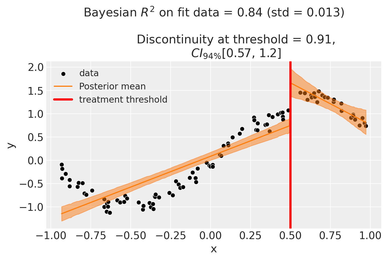
}Fit a flexible trend on each side of the cutoff with a treatment indicator; the indicator's full posterior is the discontinuity. Reports a 94% credible interval and refits on a narrow window to show how the estimate moves with bandwidth — the whole RD ballgame.
Input · what goes in
A running variable with a known threshold, a binary treatment that switches on at the cutoff, and an outcome.
Show data format & exampleHide example
Format — x (running variable), y (outcome), treatment = 1{x ≥ cutoff}.
import causalpy as cp
result = cp.pymc_experiments.RegressionDiscontinuity(
    df, formula='y ~ 1 + x + treated', running_variable_name='x',
    treatment_threshold=0.5)
result.plot()
Pipeline · the recipe ⑂ has parallel branches
↑ Click any step in the diagram to read its logic, code, assumptions & discussion.
Running variable, threshold, outcome
Data preparation — shapes the raw inputs into what the estimator expects.
Treatment switches on at the cutoff c. Identification rests on continuity of everything else at c.
import causalpy as cp
# x running variable, cutoff c, treated = (x >= c)
- No comments on this step yet — be the first.
Log in to comment on this step.
A Bayesian model each side of the cutoff
The core estimate — where the causal quantity itself is computed.
Fit a flexible trend with a treatment indicator; the coefficient on the indicator is the discontinuity, with a prior and full posterior.
result = cp.pymc_experiments.RegressionDiscontinuity(
    df, formula='y ~ 1 + x + treated',
    running_variable_name='x', treatment_threshold=0.5)
- No comments on this step yet — be the first.
Log in to comment on this step.
Posterior & 94% credible interval for the jump
Uncertainty quantification — standard errors, intervals, and aggregation.
Instead of a single number ± SE, you get the whole posterior of the discontinuity — summarised as a credible interval.
result.summary()   # discontinuity, CI_94%
result.plot()
- No comments on this step yet — be the first.
Log in to comment on this step.
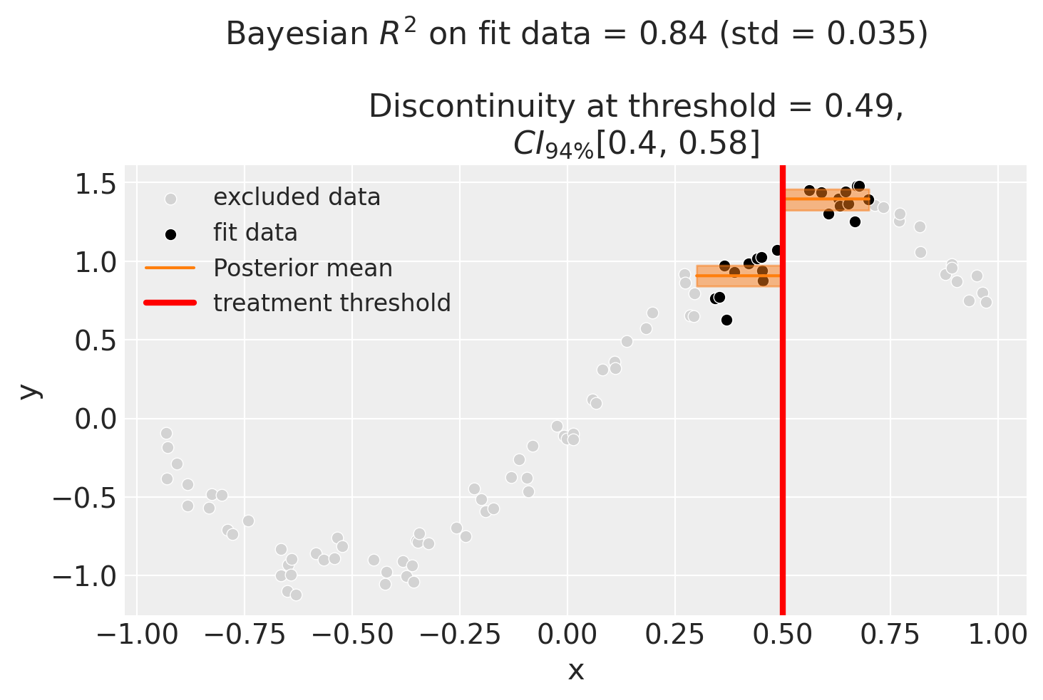
Bandwidth & functional-form sensitivity
A robustness check — does the headline result survive a different lens?
Refit on a narrow window and with different trends; a discontinuity that survives is one you can defend.
cp.pymc_experiments.RegressionDiscontinuity(
    df, ..., epsilon=0.2)   # restrict near the cutoff
- No comments on this step yet — be the first.
Log in to comment on this step.
Output · what you get 2 figures
Figures reproduced from CausalPy — PyMC Labs — unofficial community showcase; all credit to the original authors.
⚠️ Unofficial community showcase of causalpy. Not affiliated with the authors; all credit to them.
Fit a model on each side of the cutoff, put a posterior on the jump, and report a credible interval for the discontinuity — plus an honest look at how it moves with the bandwidth.
Discussion (2)
Log in to join the discussion.
A full posterior on the discontinuity beats a point estimate ± SE for communicating uncertainty to non-stats stakeholders.
Nice that the bandwidth refit is built in as a robustness step. The estimate moving with the window is the whole RD ballgame.
Exactly — I always show the narrow-window and full-sample fits next to each other so nobody thinks the number is bandwidth-free.