Synthetic control, the tidy way — weights, gaps and placebo inference (tidysynth)
@misc{tidysynth,
  title        = {tidysynth},
  author       = {Eric Dunford},
  howpublished = {\url{https://github.com/edunford/tidysynth}},
  note         = {Software / documentation}
}Build the treated unit's counterfactual as a convex blend of donors that matches its pre-treatment trajectory; read the gap as the effect. Inference is non-parametric: re-run the procedure with every donor as the placebo-treated and rank the real gap against that distribution (RMSPE ratio).
Input · what goes in
A balanced panel (unit × time) with one treated unit switching on at a known time, a donor pool, and a few pre-treatment predictors.
Show data format & exampleHide example
Format — long panel: unit, time, outcome, predictors; one treated unit after T0.
library(tidysynth)
out <- panel %>%
  synthetic_control(outcome = cigsale, unit = state, time = year,
                    i_unit = 'California', i_time = 1988) %>%
  generate_predictor(...) %>% generate_weights() %>% generate_control()
Pipeline · the recipe ⑂ has parallel branches
↑ Click any step in the diagram to read its logic, code, assumptions & discussion.
Panel, treated unit, donor pool
Data preparation — shapes the raw inputs into what the estimator expects.
Pick the treated unit and intervention time; the rest of the units form the donor pool. Identification rests on a good pre-treatment fit.
synthetic_control(outcome = cigsale, unit = state,
                  time = year, i_unit = 'California', i_time = 1988)
- No comments on this step yet — be the first.
Log in to comment on this step.
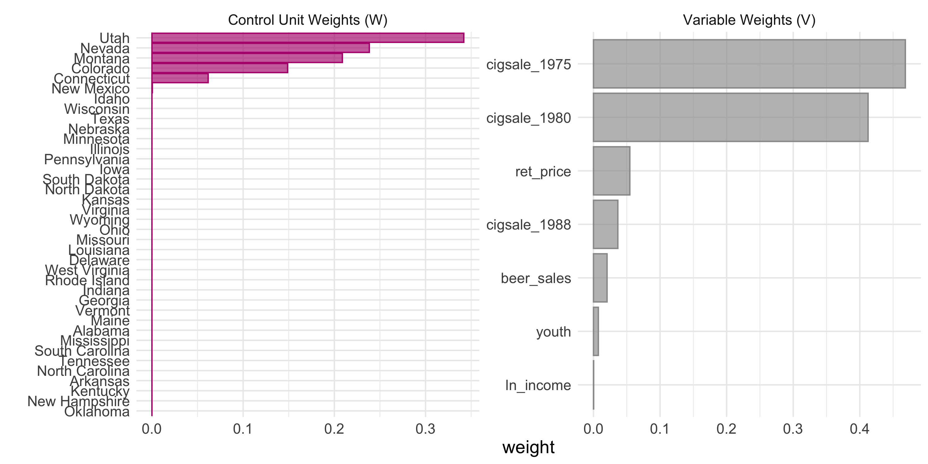
Solve for donor & predictor weights
The core estimate — where the causal quantity itself is computed.
Convex weights make the synthetic unit match the treated unit's pre-period predictors as closely as possible.
generate_weights() %>% generate_control()
- No comments on this step yet — be the first.
Log in to comment on this step.
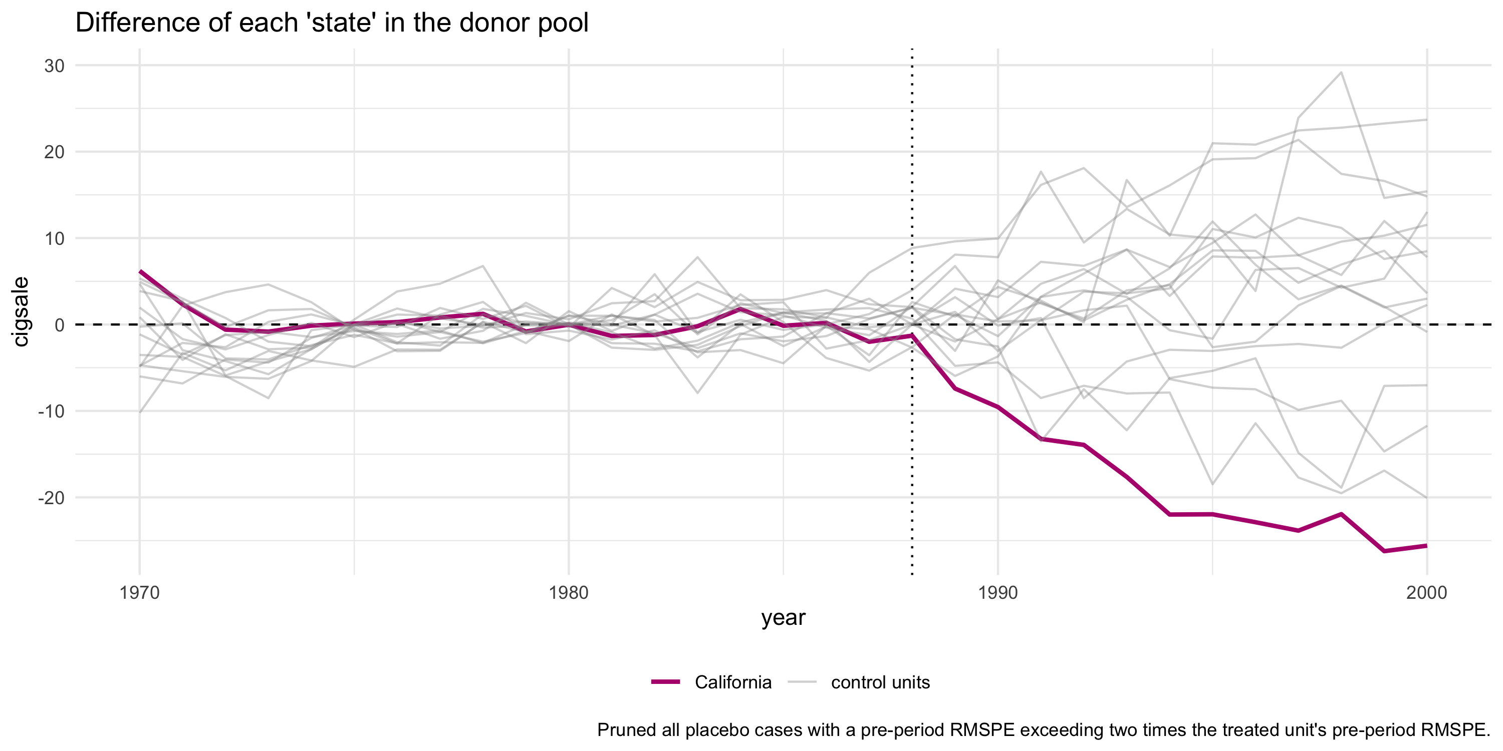
Read the gap: observed − synthetic
Reporting — turn the numbers into a figure or table a reader can act on.
The post-treatment gap between the treated unit and its synthetic twin is the estimated effect over time.
plot_trends(out); plot_differences(out)
- No comments on this step yet — be the first.
Log in to comment on this step.
Placebo permutation across donors
Uncertainty quantification — standard errors, intervals, and aggregation.
Re-run the whole procedure pretending each donor was treated; rank the real gap against that placebo distribution via the RMSPE ratio.
plot_placebos(out); plot_mspe_ratio(out)
- No comments on this step yet — be the first.
Log in to comment on this step.
Output · what you get 2 figures
Figures reproduced from tidysynth — Eric Dunford — unofficial community showcase; all credit to the original authors.
⚠️ Unofficial community showcase of tidysynth. Not affiliated with the authors; all credit to them.
Build a synthetic version of the treated unit from a convex blend of donors, read the treated-minus-synthetic gap, and test it against placebos run on every donor.
Discussion (2)
Log in to join the discussion.
The pipe-friendly API finally makes SC readable end to end. plot_placebos() as the inference step is the part people skip.
Showing the donor and predictor weights side by side is underrated — it's the honest answer to 'where does the counterfactual come from?'.
Agreed. If one donor carries 0.8 of the weight, the 'synthetic' control is basically that one unit and you should say so.