@misc{econml,
  title        = {EconML},
  author       = {ALICE},
  howpublished = {\url{https://econml.azurewebsites.net/}},
  note         = {Software / documentation}
}Cross-fit nuisance models for E[Y|X,W] and E[T|X,W], then fit a forest on the residuals so the final τ(x) is Neyman-orthogonal. The forest's adaptive weights give pointwise confidence intervals on τ(x) — heterogeneity you can actually defend.
Input · what goes in
Outcome Y, treatment T, the effect-modifiers X you want to vary the effect over, and controls W to adjust for.
Show data format & exampleHide example
Format — outcome Y, treatment T, effect-modifiers X, controls W (one row per unit).
from econml.orf import DMLOrthoForest
est = DMLOrthoForest(n_trees=1000)
est.fit(Y, T, X=X, W=W)
tau = est.effect(X_test)        # τ(x) at new points
Pipeline · the recipe ⑂ has parallel branches
↑ Click any step in the diagram to read its logic, code, assumptions & discussion.
Split features: effect-modifiers X vs controls W
Data preparation — shapes the raw inputs into what the estimator expects.
Decide what the effect is allowed to vary over (X) and what is merely confounding to adjust for (W). The target is the CATE.
# Y outcome, T treatment, X effect modifiers, W controls
- No comments on this step yet — be the first.
Log in to comment on this step.
Partial out nuisance (Neyman-orthogonal DML)
The core estimate — where the causal quantity itself is computed.
Cross-fit flexible models for E[Y|X,W] and E[T|X,W]; regress the residuals so first-stage error doesn't bias the effect.
from econml.dml import CausalForestDML
est = CausalForestDML().fit(Y, T, X=X, W=W)
- No comments on this step yet — be the first.
Log in to comment on this step.
Forest-weighted local effect τ(x)
Heterogeneity — who is affected, and by how much, not just on average.
A causal/orthogonal forest defines adaptive weights α_i(x); the effect at x solves a locally-weighted residual moment.
tau = est.effect(X_test)
est.feature_importances_
- No comments on this step yet — be the first.
Log in to comment on this step.
Confidence intervals for τ(x)
Uncertainty quantification — standard errors, intervals, and aggregation.
Honest forests / bootstrap-of-little-bags give pointwise intervals — heterogeneity you can actually defend, not just a colourful plot.
lb, ub = est.effect_interval(X_test, alpha=0.05)
- No comments on this step yet — be the first.
Log in to comment on this step.
Output · what you get
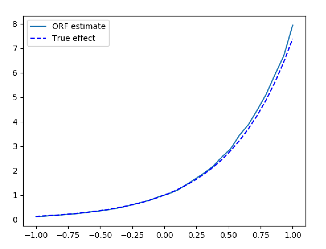
Figures reproduced from EconML — Microsoft Research (ALICE) — unofficial community showcase; all credit to the original authors.
⚠️ Unofficial community showcase of econml. Not affiliated with the authors; all credit to them.
Double machine learning with a forest final stage: partial out nuisance with flexible learners, then read the conditional effect τ(x) — with valid confidence intervals.
Discussion (2)
Log in to join the discussion.
CausalForestDML with honest intervals is my default for CATE now. The orthogonalization makes the first-stage choice forgiving.
Residual-on-residual plus forest weights — clean. How are you choosing the number of trees in practice?
Crank it until the intervals stabilise; 1–2k trees is usually plenty, and bootstrap-of-little-bags handles the inference.