@misc{grf,
  title        = {grf},
  author       = {Athey and Tibshirani and Wager},
  howpublished = {\url{https://grf-labs.github.io/grf/}},
  note         = {Software / documentation}
}K-fold cross-fitted CATEs → RATE on out-of-fold priorities → honest verdict on heterogeneity strength.
Input · what goes in
A single dataset (X, W, Y) — no separate evaluation sample needed.
Show data format & exampleHide example
Format — one row per unit. A covariate matrix X (numeric), a binary treatment W ∈ {0,1}, and an outcome Y.
  X1     X2    X3    W    Y
 0.42  -1.1   0     1   3.10
-0.07   0.6   1     0   1.85
 1.20   0.3   0     1   4.02
Pipeline · the recipe
↑ Click any step in the diagram to read its logic, code, assumptions & discussion.
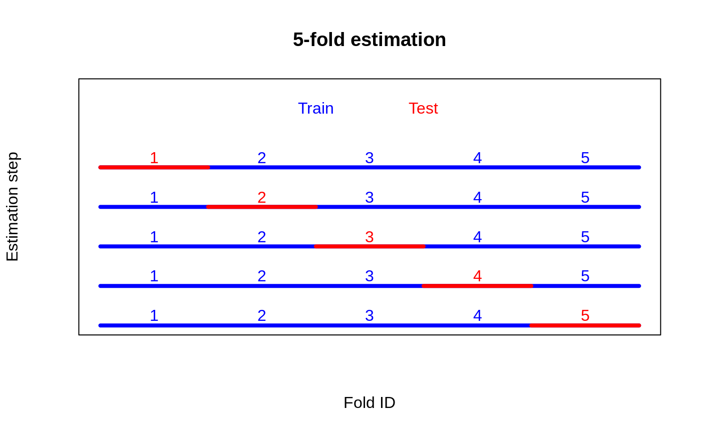
K-fold split (e.g. K = 5)
Data preparation — shapes the raw inputs into what the estimator expects.
Partition units into K folds; each unit's CATE will be predicted from a forest trained without it.
folds <- sample(rep(1:5, length.out = n)) # cross-fit by fold
- No comments on this step yet — be the first.
Log in to comment on this step.
[GRF] Regression forest
The core estimate — where the causal quantity itself is computed.
Cross-fit nuisances Y.hat, W.hat across folds.
Regression forest — Honest non-parametric regression for E[Y|X], with out-of-bag predictions and pointwise CIs.
rf <- regression_forest(X, Y)
Y.hat <- predict(rf)$predictions
- No comments on this step yet — be the first.
Log in to comment on this step.
[GRF] Causal forest
The core estimate — where the causal quantity itself is computed.
For each fold, fit on the other K−1 and predict τ̂(x) on the held-out fold.
Causal forest — Honest random forest for heterogeneous treatment effects — CATE for a binary treatment via GRF moment conditions.
cf <- causal_forest(X, Y, W)          # Y.hat, W.hat cross-fit
tau.hat <- predict(cf)$predictions    # OOB CATEs
- No comments on this step yet — be the first.
Log in to comment on this step.
[GRF] Rank-weighted ATE — RATE / AUTOC / Qini
Heterogeneity — who is affected, and by how much, not just on average.
RATE / AUTOC with the cross-fitted τ̂ as priorities — uses all the data without double-dipping.
Rank-weighted ATE — RATE / AUTOC / Qini — Evaluate how well a CATE estimate prioritizes treatment: TOC curve, AUTOC and Qini with confidence intervals.
rate <- rank_average_treatment_effect(eval.forest, priorities = tau.hat)
plot(rate)                          # TOC curve
rate$estimate / rate$std.err        # AUTOC z-stat
- No comments on this step yet — be the first.
Log in to comment on this step.
TOC curve + bootstrap CI
Reporting — turn the numbers into a figure or table a reader can act on.
Plot the curve; report whether AUTOC is bounded away from zero.
- No comments on this step yet — be the first.
Log in to comment on this step.
Output · what you get 2 figures
Figures reproduced from grf — Athey, Tibshirani & Wager — unofficial community showcase; all credit to the original authors.
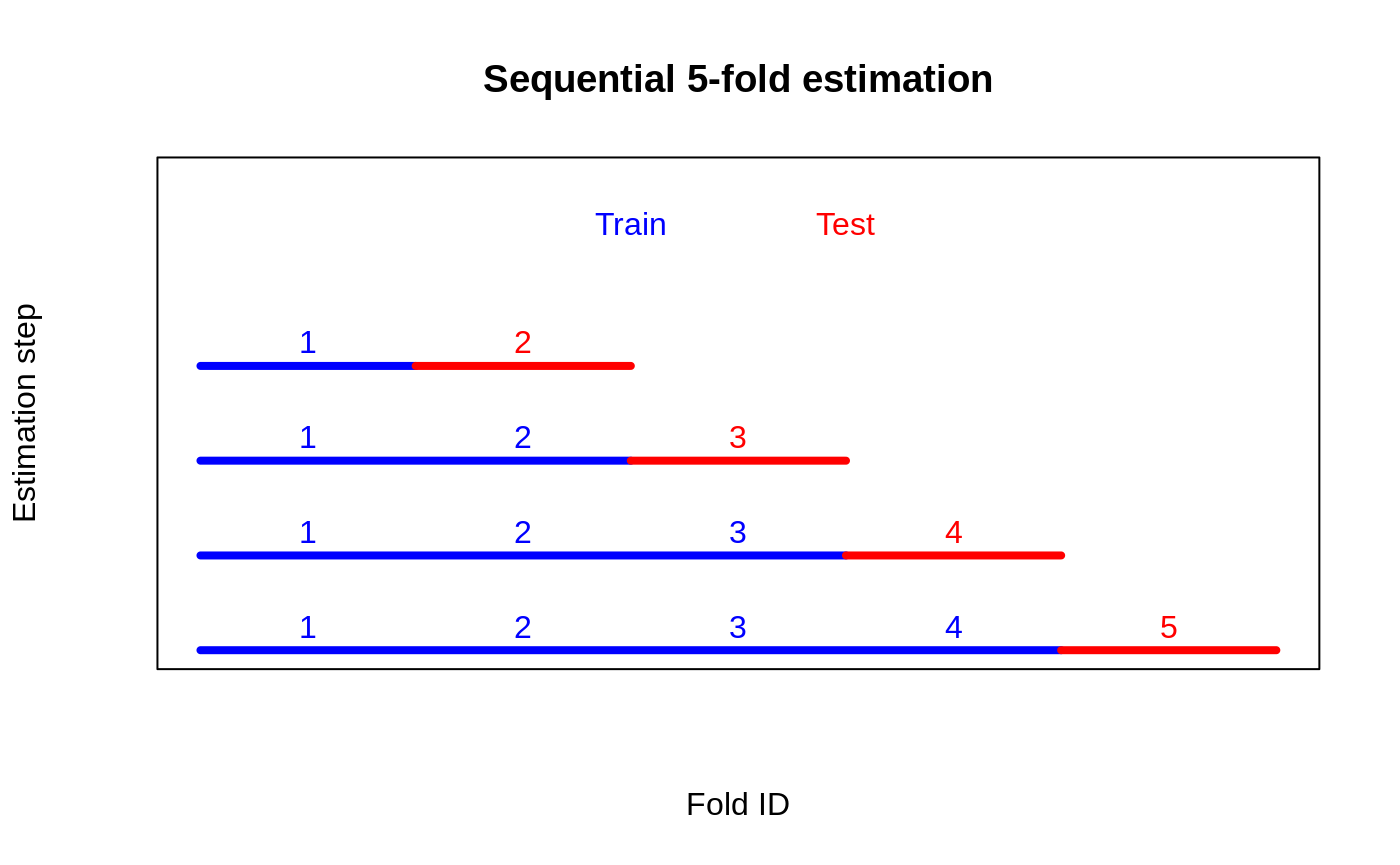
The GRF 'Cross-fold validation of heterogeneity' tutorial. Sample-splitting RATE wastes half the data; K-fold cross-fitting fixes that while keeping the priorities out-of-sample at every unit. Unofficial summary.
Discussion (0)
Log in to join the discussion.