Goodman-Bacon decomposition: what your TWFE estimate is averaging (bacondecomp)
@misc{bacondecomp,
  title        = {bacondecomp},
  author       = {2021},
  howpublished = {\url{https://github.com/evanjflack/bacondecomp}},
  note         = {Software / documentation}
}Your headline TWFE coefficient is a variance-weighted average of every 2×2 DiD inside the panel — including the dangerous 'later vs. earlier treated' comparisons that use already-treated units as controls. This decomposes those weights so you can see when the average is trustworthy.
Input · what goes in
A staggered-adoption panel: units adopting treatment at different times, with a binary treatment indicator.
Show data format & exampleHide example
Format — long panel: unit, time, outcome y, treatment treated (0/1, absorbing).
library(bacondecomp)
df_bacon <- bacon(y ~ treated, data = panel,
                  id_var = 'unit', time_var = 'year')
Pipeline · the recipe ⑂ has parallel branches
↑ Click any step in the diagram to read its logic, code, assumptions & discussion.
A staggered-adoption panel
Data preparation — shapes the raw inputs into what the estimator expects.
Units switch treatment on at different dates. The TWFE coefficient you'd normally report hides a lot of structure.
# unit, year, y, treated (0/1, turns on and stays on)
- No comments on this step yet — be the first.
Log in to comment on this step.
Decompose into 2×2 comparisons
A pre-flight check — run this before trusting any estimate downstream.
Every pair of timing groups forms a 2×2 DiD; TWFE is their variance-weighted average.
df_bacon <- bacon(y ~ treated, data = panel,
                  id_var = 'unit', time_var = 'year')
- No comments on this step yet — be the first.
Log in to comment on this step.
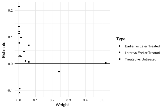
Spot the forbidden comparisons
A robustness check — does the headline result survive a different lens?
'Later vs earlier treated' uses already-treated units as controls — under dynamic effects this term is biased and can carry negative weight.
library(ggplot2)
ggplot(df_bacon, aes(weight, estimate, color = type)) + geom_point()
- No comments on this step yet — be the first.
Log in to comment on this step.
Read β as a weighted average
Reporting — turn the numbers into a figure or table a reader can act on.
If the dangerous comparisons carry real weight, prefer a modern estimator (Callaway-Sant'Anna, did2s) over plain TWFE.
weighted.mean(df_bacon$estimate, df_bacon$weight)
- No comments on this step yet — be the first.
Log in to comment on this step.
Output · what you get
Figures reproduced from bacondecomp — Flack; Goodman-Bacon (2021) — unofficial community showcase; all credit to the original authors.
⚠️ Unofficial community showcase of bacondecomp. Not affiliated with the authors; all credit to them.
A two-way fixed-effects DiD is a weighted average of all possible 2×2 comparisons — including 'forbidden' ones that use already-treated units as controls. This shows you the weights.
Discussion (2)
Log in to join the discussion.
Every staggered-DiD paper should print this plot. Once you see the 'later vs earlier treated' weight, you can't unsee the TWFE problem.
Great diagnostic, but it's a diagnosis not a cure — pair it with Callaway-Sant'Anna or did2s when the bad comparisons carry weight.