@misc{matchit,
  title        = {MatchIt},
  author       = {Ho and Imai and King and Stuart},
  howpublished = {\url{https://kosukeimai.github.io/MatchIt/}},
  note         = {Software / documentation}
}Preprocess by matching so groups are comparable, check balance, then estimate the effect on the matched sample — design before analysis.
Input · what goes in
A binary treatment and the covariates to match on (Lalonde job-training data).
Show data format & exampleHide example
Format — one row per unit: treatment W ∈ {0,1} and covariates X.
  W  age educ   race   re74  re75
  1   37   11  black     0     0
  0   30   12  white  4100  3800
Pipeline · the recipe
↑ Click any step in the diagram to read its logic, code, assumptions & discussion.
Treatment W + covariates X
Data preparation — shapes the raw inputs into what the estimator expects.
Binary treatment plus the covariates to match on.
data("lalonde", package = "MatchIt")
- No comments on this step yet — be the first.
Log in to comment on this step.
[MatchIt] Matching for causal inference — matchit()
The core estimate — where the causal quantity itself is computed.
Nearest-neighbor matching on the estimated propensity score.
Matching for causal inference — matchit() — Nearest-neighbor, optimal, full, and genetic matching to preprocess data so treated and control groups are comparable before estimating effects.
m <- matchit(treat ~ age + educ + race + re74 + re75, lalonde, method = "nearest")
- No comments on this step yet — be the first.
Log in to comment on this step.
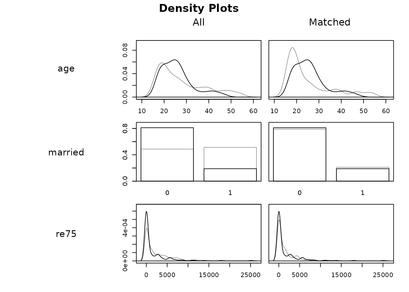
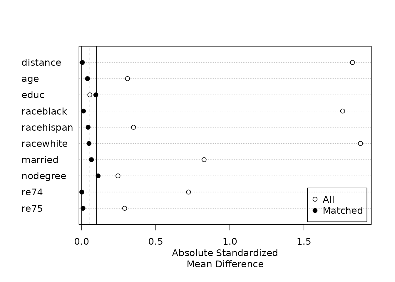
Assess balance (summary / plot)
A pre-flight check — run this before trusting any estimate downstream.
Check standardized mean differences and eCDF/QQ plots on the matched sample.
summary(m); plot(m, type = "jitter")
- No comments on this step yet — be the first.
Log in to comment on this step.
Estimate the effect on matched data
Reporting — turn the numbers into a figure or table a reader can act on.
Fit the outcome model on match.data() with cluster-robust SEs.
fit <- lm(re78 ~ treat, data = match.data(m), weights = weights)
- No comments on this step yet — be the first.
Log in to comment on this step.
Output · what you get 3 figures

Figures reproduced from MatchIt — Ho, Imai, King & Stuart — unofficial community showcase; all credit to the original authors.
The MatchIt vignette (Lalonde). Match, assess balance, and only then estimate. Unofficial summary.
Discussion (2)
Log in to join the discussion.
Matching as the design stage — outcome-free — is the discipline people skip. MatchIt makes it the path of least resistance.
And match.data() → any outcome model. Pairs perfectly with cobalt for the balance plots.
Nearest, optimal, full, genetic — all behind one matchit() call. Great teaching tool.