Mendelian randomization: genes as instruments for a causal effect (TwoSampleMR)
@misc{twosamplemr,
  title        = {TwoSampleMR},
  author       = {Hemani and Davey Smith and others},
  howpublished = {\url{https://mrcieu.github.io/TwoSampleMR/}},
  note         = {Software / documentation}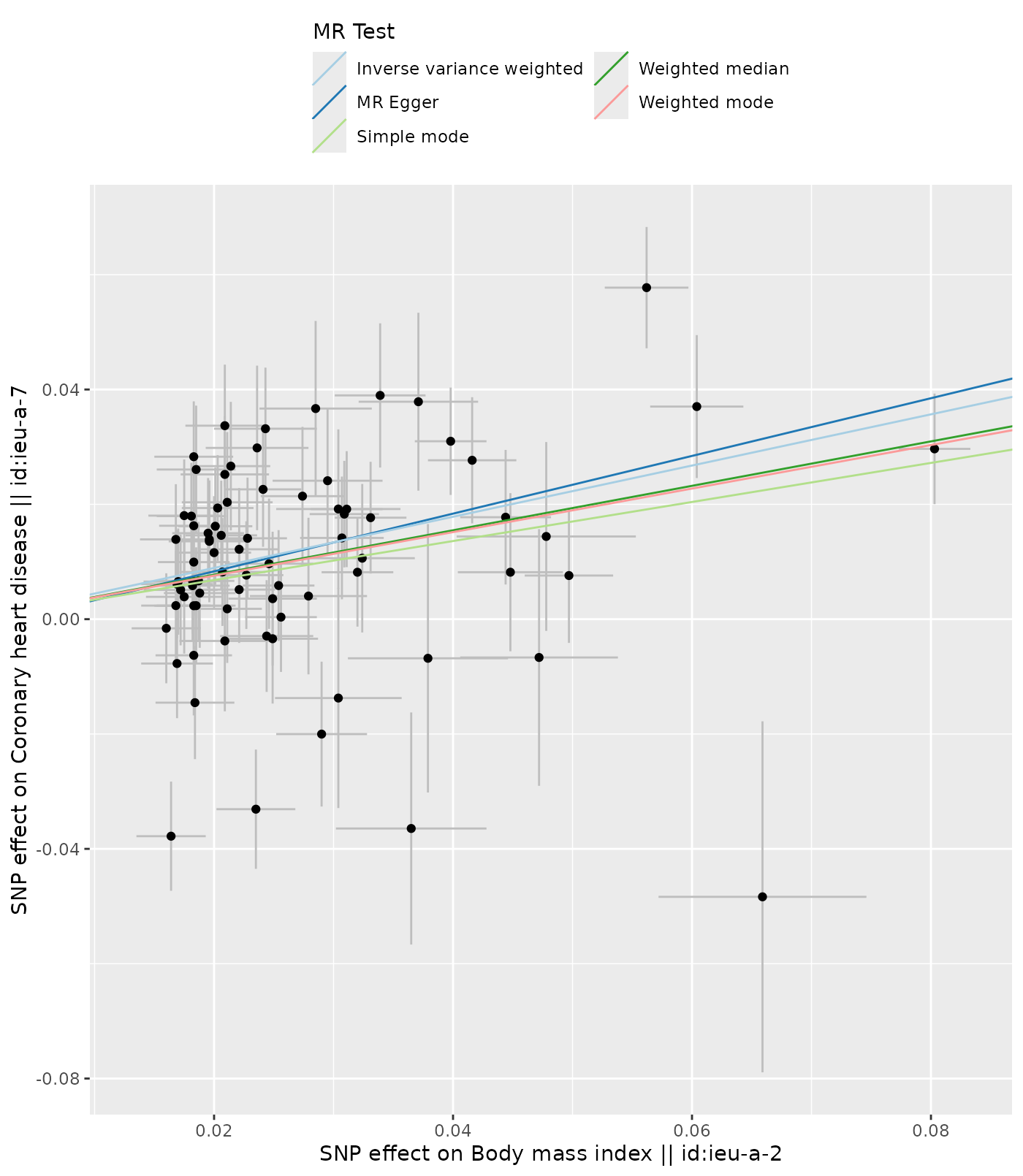
}Use genetic variants as instruments for an exposure → outcome effect from GWAS summary stats. IVW pools per-SNP Wald ratios by precision; MR-Egger tests directional pleiotropy via the intercept; weighted-median and mode are robust to a chunk of invalid instruments.
Input · what goes in
GWAS summary statistics: for each SNP, its effect on the exposure and on the outcome (with standard errors), harmonised to a common effect allele.
Show data format & exampleHide example
Format — per-SNP effects on exposure and outcome, harmonised.
library(TwoSampleMR)
exp <- extract_instruments('ieu-a-2')           # BMI instruments
out <- extract_outcome_data(exp$SNP, 'ieu-a-7')  # coronary heart disease
dat <- harmonise_data(exp, out)
res <- mr(dat)
Pipeline · the recipe ⑂ has parallel branches
↑ Click any step in the diagram to read its logic, code, assumptions & discussion.
Harmonise SNP–exposure & SNP–outcome effects
Data preparation — shapes the raw inputs into what the estimator expects.
Each SNP is a candidate instrument. Align effect alleles across the two GWAS so the signs are comparable.
dat <- harmonise_data(exp, out)
- No comments on this step yet — be the first.
Log in to comment on this step.
Check instrument strength
A pre-flight check — run this before trusting any estimate downstream.
Weak instruments bias MR. Read the variance explained and the F-statistic before trusting anything.
# per-SNP F = (beta/se)^2; overall F from R^2
- No comments on this step yet — be the first.
Log in to comment on this step.
Inverse-variance weighted estimate
The core estimate — where the causal quantity itself is computed.
Combine the per-SNP Wald ratios, weighting by precision — the IVW estimate.
mr(dat, method_list = c('mr_ivw'))
- No comments on this step yet — be the first.
Log in to comment on this step.
Pleiotropy-robust: MR-Egger, weighted median
A robustness check — does the headline result survive a different lens?
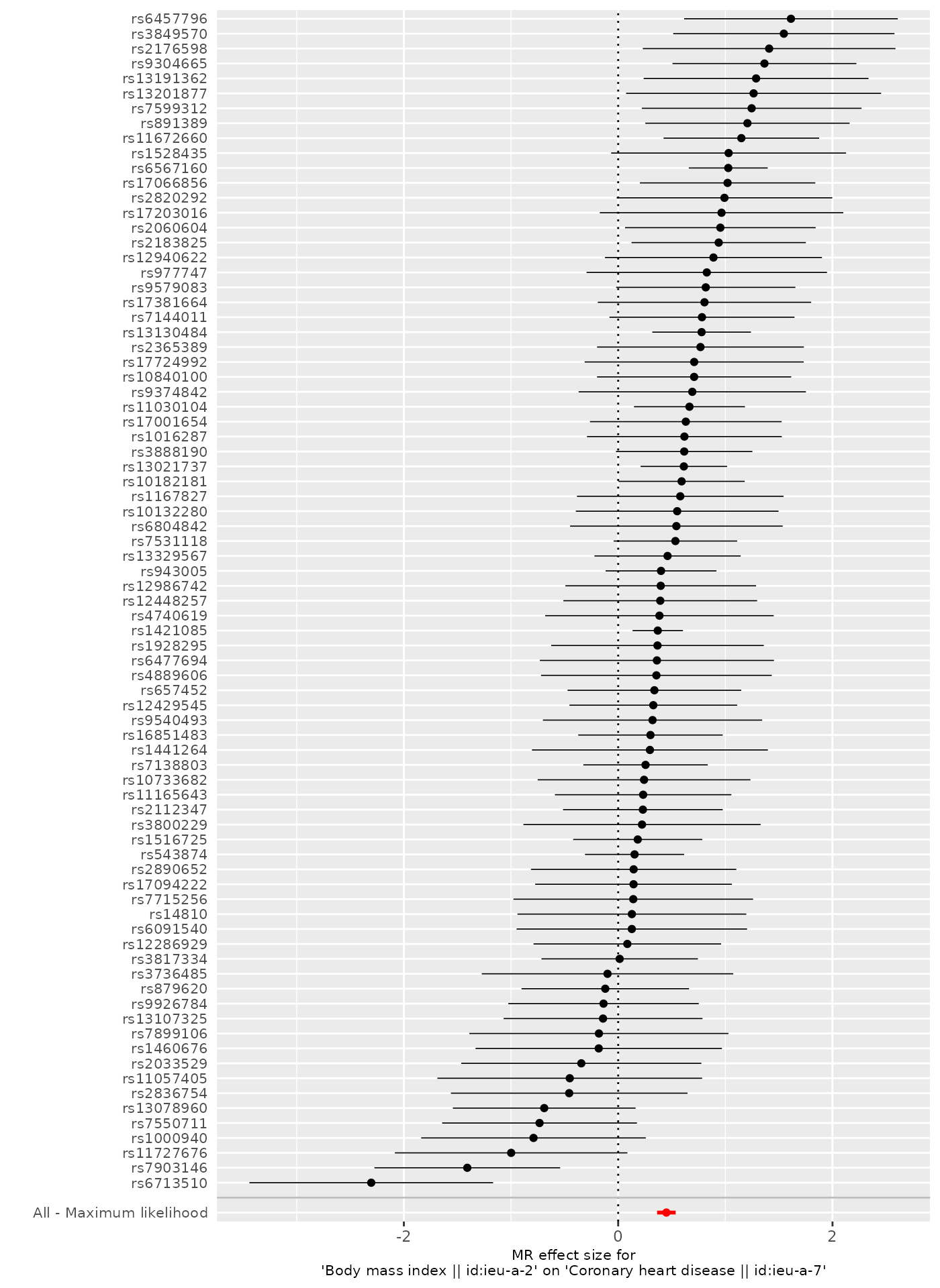
If instruments affect the outcome through other paths, IVW is biased. The MR-Egger intercept tests directional pleiotropy; weighted median/mode are robust to some invalid instruments.
mr(dat, method_list = c('mr_egger_regression',
                         'mr_weighted_median'))
- No comments on this step yet — be the first.
Log in to comment on this step.
Output · what you get 2 figures
Figures reproduced from TwoSampleMR — MRC IEU (Hemani, Davey Smith et al.) — unofficial community showcase; all credit to the original authors.
⚠️ Unofficial community showcase of twosamplemr. Not affiliated with the authors; all credit to them.
Use genetic variants as instruments to estimate the causal effect of an exposure on an outcome from GWAS summary data — with IVW plus pleiotropy-robust MR-Egger and weighted-median checks.
Discussion (2)
Log in to join the discussion.
Genes as instruments is the cleanest natural experiment we get — but the MR-Egger intercept and weighted-median checks are non-negotiable. Pleiotropy is everywhere.
The scatter with all five estimator slopes on one plot is the right way to show robustness at a glance. Saved.
Agreed — if IVW and Egger disagree wildly, that's the figure that makes the pleiotropy story obvious to a reviewer.