@misc{grf,
  title        = {grf},
  author       = {Athey and Tibshirani and Wager},
  howpublished = {\url{https://grf-labs.github.io/grf/}},
  note         = {Software / documentation}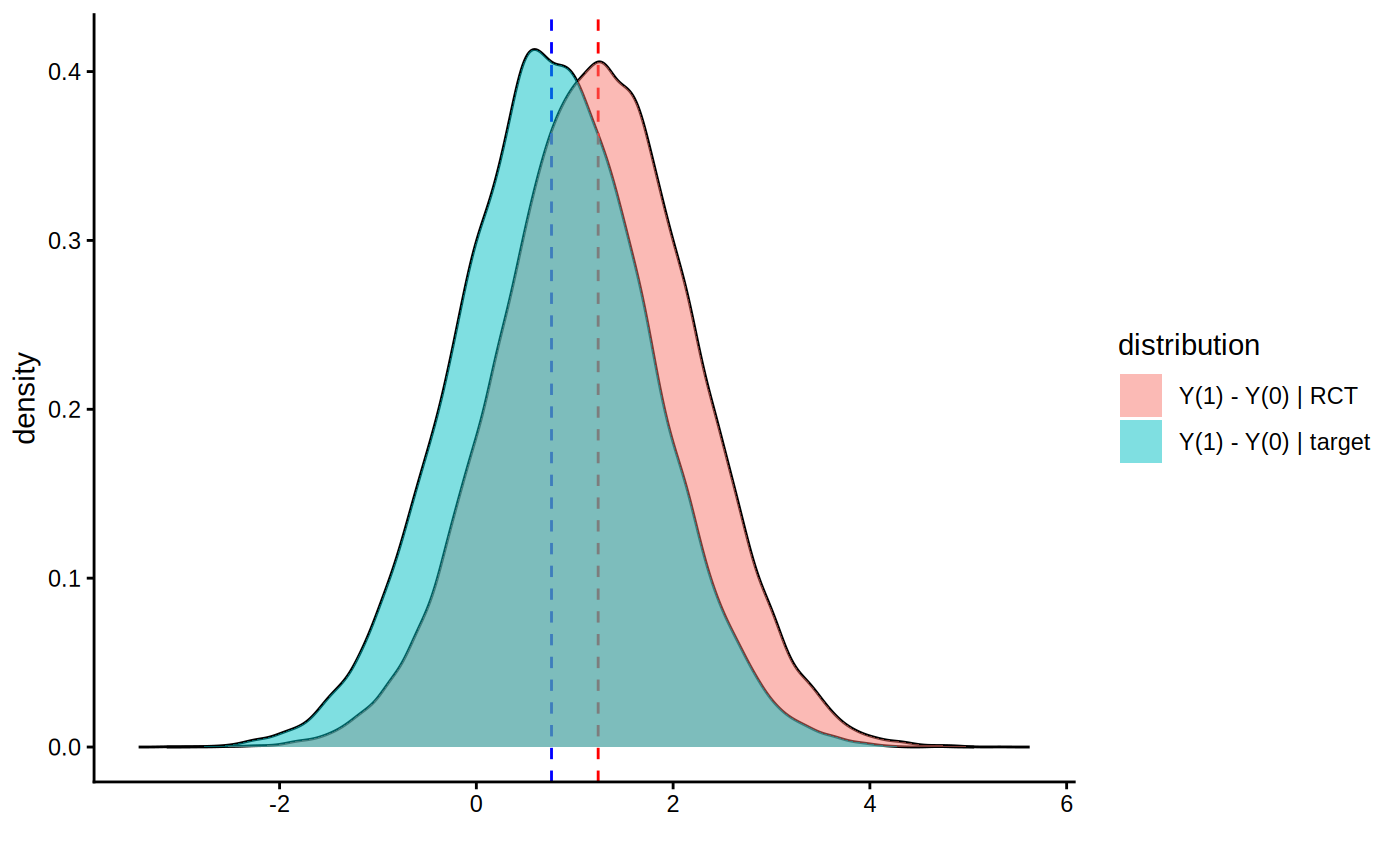
}Train a causal forest on the source sample → reweight AIPW to a target population → report transported ATE.
Input · what goes in
A source RCT (X, W, Y) and a target population's covariates X_test.
Show data format & exampleHide example
Format — one row per unit. A covariate matrix X (numeric), a binary treatment W ∈ {0,1}, and an outcome Y.
  X1     X2    X3    W    Y
 0.42  -1.1   0     1   3.10
-0.07   0.6   1     0   1.85
 1.20   0.3   0     1   4.02
Pipeline · the recipe
↑ Click any step in the diagram to read its logic, code, assumptions & discussion.
[GRF] Causal forest
The core estimate — where the causal quantity itself is computed.
Fit on the source sample where treatment varies.
Causal forest — Honest random forest for heterogeneous treatment effects — CATE for a binary treatment via GRF moment conditions.
cf <- causal_forest(X, Y, W)          # Y.hat, W.hat cross-fit
tau.hat <- predict(cf)$predictions    # OOB CATEs
- No comments on this step yet — be the first.
Log in to comment on this step.
[GRF] AIPW average treatment effect
Uncertainty quantification — standard errors, intervals, and aggregation.
Reweight AIPW scores to the target covariate distribution (target.sample / target.weights).
AIPW average treatment effect — Doubly-robust ATE / ATT / ATC / overlap-weighted effect from a trained causal forest, via augmented IPW.
average_treatment_effect(cf, target.sample = "all")      # ATE
average_treatment_effect(cf, target.sample = "treated")  # ATT
- No comments on this step yet — be the first.
Log in to comment on this step.
Transported ATE + overlap caveats
Reporting — turn the numbers into a figure or table a reader can act on.
Report the target-population ATE and flag regions of thin overlap where it's extrapolating.
- No comments on this step yet — be the first.
Log in to comment on this step.
Output · what you get
Figures reproduced from grf — Athey, Tibshirani & Wager — unofficial community showcase; all credit to the original authors.
The GRF 'Estimating ATEs on a new target population' tutorial. Uses the forest's doubly-robust scores with target weights to transport the effect, and is honest about overlap. Unofficial summary.
Discussion (0)
Log in to join the discussion.