Workflow·5 steps·branched

Staggered DiD done three ways (did · did2s · fixest)

@tianzhuqin D · Jun 4, 2026 · 728 views

Summary by StatsDoge

My side-by-side for staggered adoption: Callaway–Sant'Anna vs Gardner's two-stage vs Sun–Abraham — do the event studies agree?

Input · what goes in

A long, staggered panel: unit id, period, the unit's first-treatment period (cohort), and an outcome.

Show data format & exampleHide example

Format — one row per (unit, period). cohort = first treated period (0 = never).

 id  period  cohort   y
  1     2004     2006   8.1
  1     2005     2006   8.4
  2     2004        0   7.9

Pipeline · the recipe ⑂ has parallel branches

↑ Click any step in the diagram to read its logic, code, assumptions & discussion.

Data prep

Build the staggered panel

Data preparation — shapes the raw inputs into what the estimator expects.

What happens here

One row per (unit, period); never-treated units get cohort 0 / Inf.

Reads from the input data Feeds into the final output

Key code

# id · period · cohort (first treated) · y
head(panel)

Discussion on this step (0)

No comments on this step yet — be the first.

Estimation

att_gt() — Callaway & Sant'Anna

The core estimate — where the causal quantity itself is computed.

What happens here

ATT(g,t) against not-yet-treated controls, aggregated to a dynamic event study.

Formula

\mathrm{ATT}(g,t)=\mathbb{E}\!\left[\,Y_t(g)-Y_t(\infty)\mid G=g\,

Reads from the input data Feeds into the final output

Key code

att <- att_gt("y","period","id","cohort", data=panel)
es_cs <- aggte(att, type="dynamic")

Reference / docs ↗

Discussion on this step (0)

No comments on this step yet — be the first.

Estimation

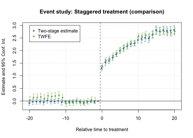
did2s() — Gardner two-stage

The core estimate — where the causal quantity itself is computed.

What happens here

Gardner's two-stage estimator on the same panel — fast, timing-robust.

Reads from the input data Feeds into the final output

Key code

es_2s <- did2s(panel, yname="y", first_stage=~0|id+period,
               second_stage=~i(rel_year), treatment="treat", cluster_var="id")

Reference / docs ↗

Discussion on this step (0)

No comments on this step yet — be the first.

Estimation

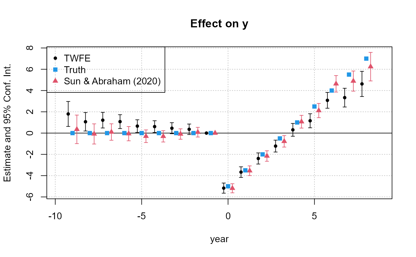
sunab() — Sun & Abraham (fixest)

The core estimate — where the causal quantity itself is computed.

What happens here

Interaction-weighted Sun–Abraham event study via fixest.

Reads from the input data Feeds into the final output

Key code

es_sa <- feols(y ~ sunab(cohort, period) | id + period, panel)

Reference / docs ↗

Discussion on this step (0)

No comments on this step yet — be the first.

Reporting

Overlay the three event studies

Reporting — turn the numbers into a figure or table a reader can act on.

What happens here

Plot CS, did2s and Sun–Abraham together; agreement is the evidence.

Reads from the input data Feeds into the final output

Key code

# overlay es_cs, es_2s, es_sa on one event-time axis

Discussion on this step (0)

No comments on this step yet — be the first.

Output · what you get 3 figures

Fig 1Callaway–Sant'Anna event study (aggte, dynamic): effect by length of exposure with pre-trend checks.

Fig 2did2s vs TWFE vs Callaway–Sant'Anna — the estimators side by side.

Fig 3Sun–Abraham (fixest) tracking the true effect where naive TWFE drifts.

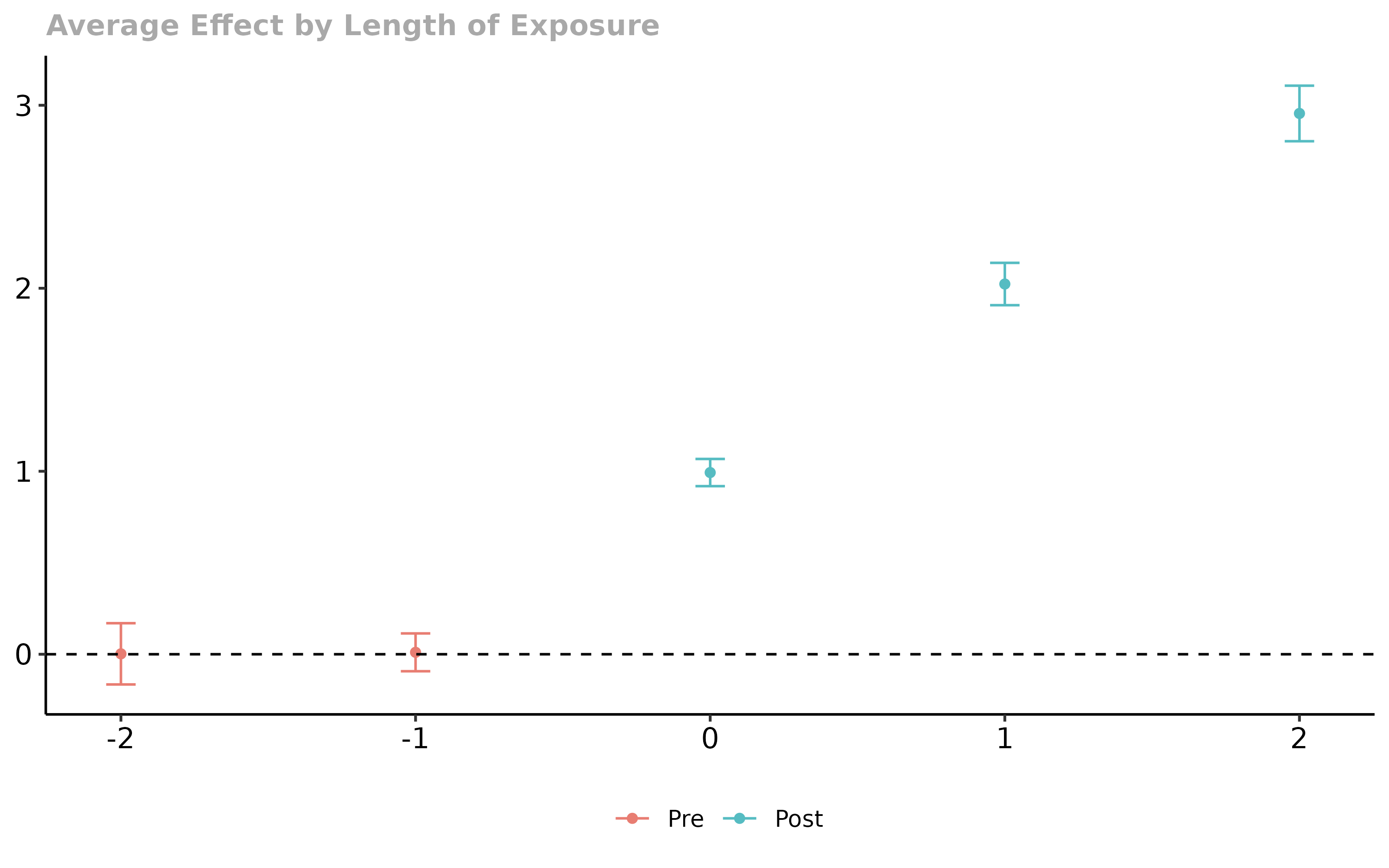
Figures reproduced from the package's official documentation — unofficial community showcase; all credit to the original authors.

Personal recipe — figures are from each package's public docs; this is my own composition, not affiliated with the package authors.

When treatment rolls out at different times, plain TWFE is biased. I run three modern estimators on the same panel and overlay their event studies — if they agree, I trust the dynamics.

Staggered DiD done three ways (did · did2s · fixest)

Input · what goes in

Pipeline · the recipe ⑂ has parallel branches

Output · what you get 3 figures

Discussion (0)