@misc{doubleml,
  title        = {DoubleML},
  author       = {Bach and Chernozhukov and Kurz and Spindler},
  howpublished = {\url{https://docs.doubleml.org/}},
  note         = {Software / documentation}
}Effect of 401(k) eligibility on net assets via PLR / IRM / IIVM with cross-fit ML nuisances — four learners, one honest comparison.
Input · what goes in
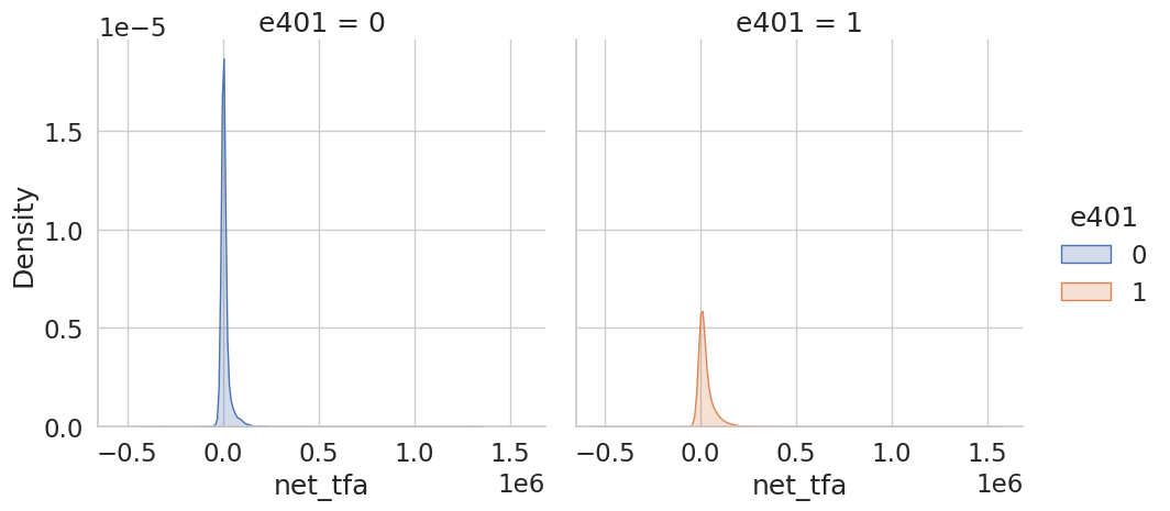
Outcome (net financial assets), treatment (401(k) eligibility), covariates, and an instrument (eligibility) for the IV model.
Show data format & exampleHide example
Format — one row per household: outcome y, treatment d, covariates X (and instrument z for IIVM).
  net_tfa(y)  e401(d)  age  inc    educ  ...
   12000        1      41  38k    13
    -400        0      53  21k    11
Pipeline · the recipe ⑂ has parallel branches
↑ Click any step in the diagram to read its logic, code, assumptions & discussion.
Build DoubleMLData (y, d, X, z)
Data preparation — shapes the raw inputs into what the estimator expects.
Declare outcome, treatment, covariates and (optionally) an instrument.
dml_data = dml.DoubleMLData(df, y_col='net_tfa', d_cols='e401', x_cols=X)
- No comments on this step yet — be the first.
Log in to comment on this step.
Choose ML learners for the nuisances
Data preparation — shapes the raw inputs into what the estimator expects.
e.g. random forest / lasso for E[Y|X] and E[D|X]; estimated by cross-fitting.
ml_l = RandomForestRegressor(); ml_m = RandomForestClassifier()
- No comments on this step yet — be the first.
Log in to comment on this step.
[DoubleML] Double/debiased ML — PLR / IRM / IIVM
The core estimate — where the causal quantity itself is computed.
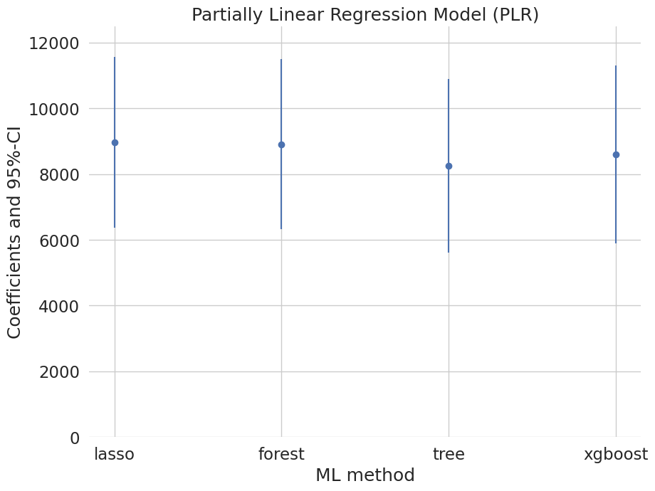
Partially-linear regression (PLR) for the average effect, with orthogonal scores.
Double/debiased ML — PLR / IRM / IIVM — Neyman-orthogonal, cross-fitted estimation of treatment effects with arbitrary ML nuisance learners.
dml.DoubleMLPLR(dml_data, ml_l, ml_m).fit().summary
- No comments on this step yet — be the first.
Log in to comment on this step.
IRM / IIVM cross-checks
A robustness check — does the headline result survive a different lens?
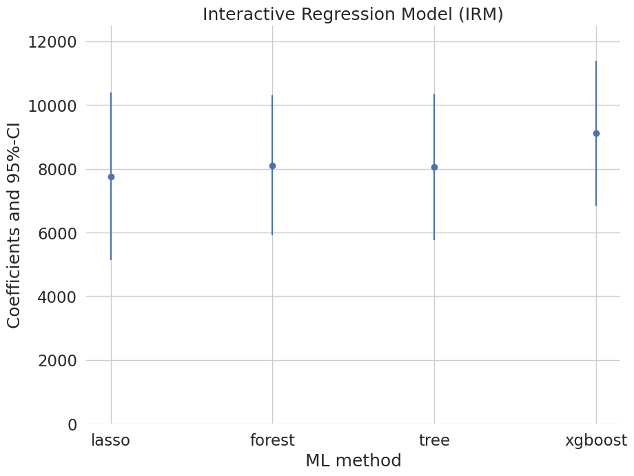
Interactive (IRM) and IV (IIVM) models as alternative identifications.
dml.DoubleMLIRM(dml_data, ml_g, ml_m).fit()
- No comments on this step yet — be the first.
Log in to comment on this step.
Coefficient comparison plot
Reporting — turn the numbers into a figure or table a reader can act on.
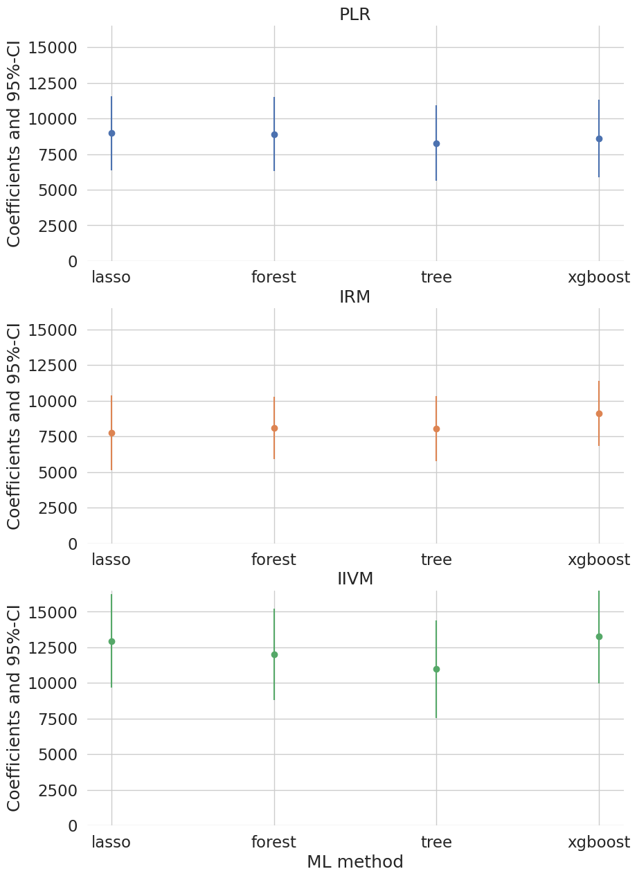
Compare estimates across PLR/IRM/IIVM × learners with 95% confidence intervals.
# error-bar plot of coef ± 1.96·se per model × learner
- No comments on this step yet — be the first.
Log in to comment on this step.
Output · what you get 4 figures
Figures reproduced from DoubleML — Bach, Chernozhukov, Kurz & Spindler — unofficial community showcase; all credit to the original authors.
The DoubleML 401(k) example (SIPP data). Build the DoubleMLData, choose ML learners, and estimate the effect three ways (PLR / IRM / IIVM). Unofficial summary.
Discussion (3)
Log in to join the discussion.
Cross-fitting + Neyman-orthogonal scores = you can throw any ML at the nuisances and still get √n-consistent, valid CIs. This is the way.
And it generalizes AIPW cleanly. PLR for a quick read, IRM when effects are nonlinear in X.
The 401(k) example is the perfect teaching case. Same data, three orthogonal scores, sane answers.
Pairs beautifully with GRF: DoubleML for the average, causal forest for the heterogeneity.