Workflow·4 steps·branched

Sensitivity analysis for unobserved confounding (sensemakr)

@sensemakr ✓ P D · Jun 3, 2026 · 790 views

@misc{sensemakr,
  title        = {sensemakr},
  author       = {Cinelli and Hazlett},
  howpublished = {\url{https://github.com/carloscinelli/sensemakr}},
  note         = {Software / documentation}
}

Summary by StatsDoge

Don't just assume no unobserved confounding — quantify it: robustness value + contour plots benchmarked against your real covariates.

Input · what goes in

A fitted OLS outcome model: outcome ~ treatment + observed covariates.

Show data format & exampleHide example

Format — one row per unit: outcome Y, treatment D, covariates X.

   Y     D   X1   X2  ...
 3.2     1  0.4  -1.1
 1.8     0 -0.1   0.6

Pipeline · the recipe ⑂ has parallel branches

↑ Click any step in the diagram to read its logic, code, assumptions & discussion.

Data prep

Fit the OLS outcome model

Data preparation — shapes the raw inputs into what the estimator expects.

What happens here

Outcome ~ treatment + observed covariates.

Reads from the input data Feeds into #2

Key code

fit <- lm(peacefactor ~ directlyharmed + age + female + ..., data = darfur)

Discussion on this step (0)

No comments on this step yet — be the first.

Estimation

[sensemakr] Sensitivity to unobserved confounding

The core estimate — where the causal quantity itself is computed.

What happens here

Compute the robustness value and partial-R² sensitivity statistics.

Formula

\mathrm{RV}_q= frac12ig(\sqrt{f_q^4+4f_q^2}-f_q^2ig),\ \ f_q=q\,|t_{\hateta}|/\sqrt{df}

The estimator

Sensitivity to unobserved confounding — How strong would an unobserved confounder have to be to overturn your OLS result? Robustness values + contour plots, no extra assumptions.

OTHER Code @ HEAD ↗ Paper ↗

Reads from #1 Feeds into #3#4

Key code

s <- sensemakr(fit, treatment = "directlyharmed", benchmark_covariates = "female", kd = 1:3)

Discussion on this step (0)

No comments on this step yet — be the first.

Reporting

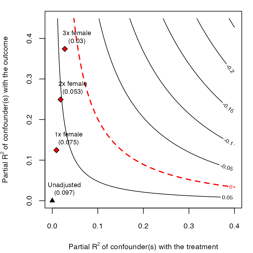
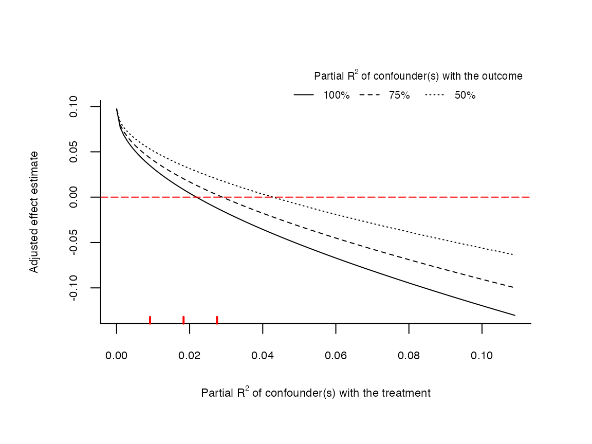
Contour plot — point estimate

Reporting — turn the numbers into a figure or table a reader can act on.

What happens here

How strong must a confounder be (vs observed covariates) to drive the estimate to zero?

Reads from #2 Feeds into the final output

Key code

plot(s)

Reference / docs ↗

Discussion on this step (0)

No comments on this step yet — be the first.

Reporting

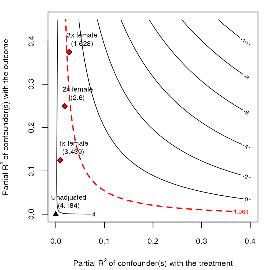
Contour plot — t-value

Reporting — turn the numbers into a figure or table a reader can act on.

What happens here

Same, for statistical significance.

Reads from #2 Feeds into the final output

Key code

plot(s, sensitivity.of = "t-value")

Discussion on this step (0)

No comments on this step yet — be the first.

Output · what you get 3 figures

Fig 1Contour plot of the point estimate: how strong a confounder must be (vs observed covariates) to drive it to zero.

Fig 2The same sensitivity contours, drawn for the t-value (statistical significance).

Fig 3Extreme-scenario analysis: the estimate as hypothesised confounder strength grows.

Figures reproduced from sensemakr — Cinelli & Hazlett — unofficial community showcase; all credit to the original authors.

The sensemakr vignette (Cinelli & Hazlett). Fit your model, then report how strong hidden confounding would need to be to change the conclusion. Unofficial summary.

Discussion (2)

3

@calibrator_cleo · Jun 3, 2026

Unconfoundedness is an assumption, not a fact. sensemakr makes you state HOW wrong you could be. Every observational paper should include this.

6

@nuisance_nina · Jun 3, 2026

The robustness value is such a clean one-number summary. 'A confounder would need to explain 15% of residual variance to overturn this.'
4

@ivan_iv · Jun 3, 2026

Benchmarking against observed covariates is the killer feature — 'as strong as 3× the effect of female' is interpretable.