@misc{did,
  title        = {did},
  author       = {Callaway and Sant'Anna},
  howpublished = {\url{https://bcallaway11.github.io/did/}},
  note         = {Software / documentation}
}Staggered-adoption DiD done right: group-time ATT(g,t) → event-study / group / calendar aggregations, with honest pre-trends.
Input · what goes in
A long panel with staggered treatment timing: unit id, period, the unit's first-treatment period (group), and an outcome.
Show data format & exampleHide example
Format — one row per (unit, period). first.treat = the period a unit is first treated (0 / Inf = never treated).
 id  period  first.treat   Y
  1     2004        2006    8.1
  1     2005        2006    8.4
  2     2004           0    7.9   # never treated
Pipeline · the recipe ⑂ has parallel branches
↑ Click any step in the diagram to read its logic, code, assumptions & discussion.
Build the staggered panel
Data preparation — shapes the raw inputs into what the estimator expects.
One row per (unit, period); never-treated units get group 0 / Inf.
# id · period · first.treat (group) · Y
head(panel)
- No comments on this step yet — be the first.
Log in to comment on this step.
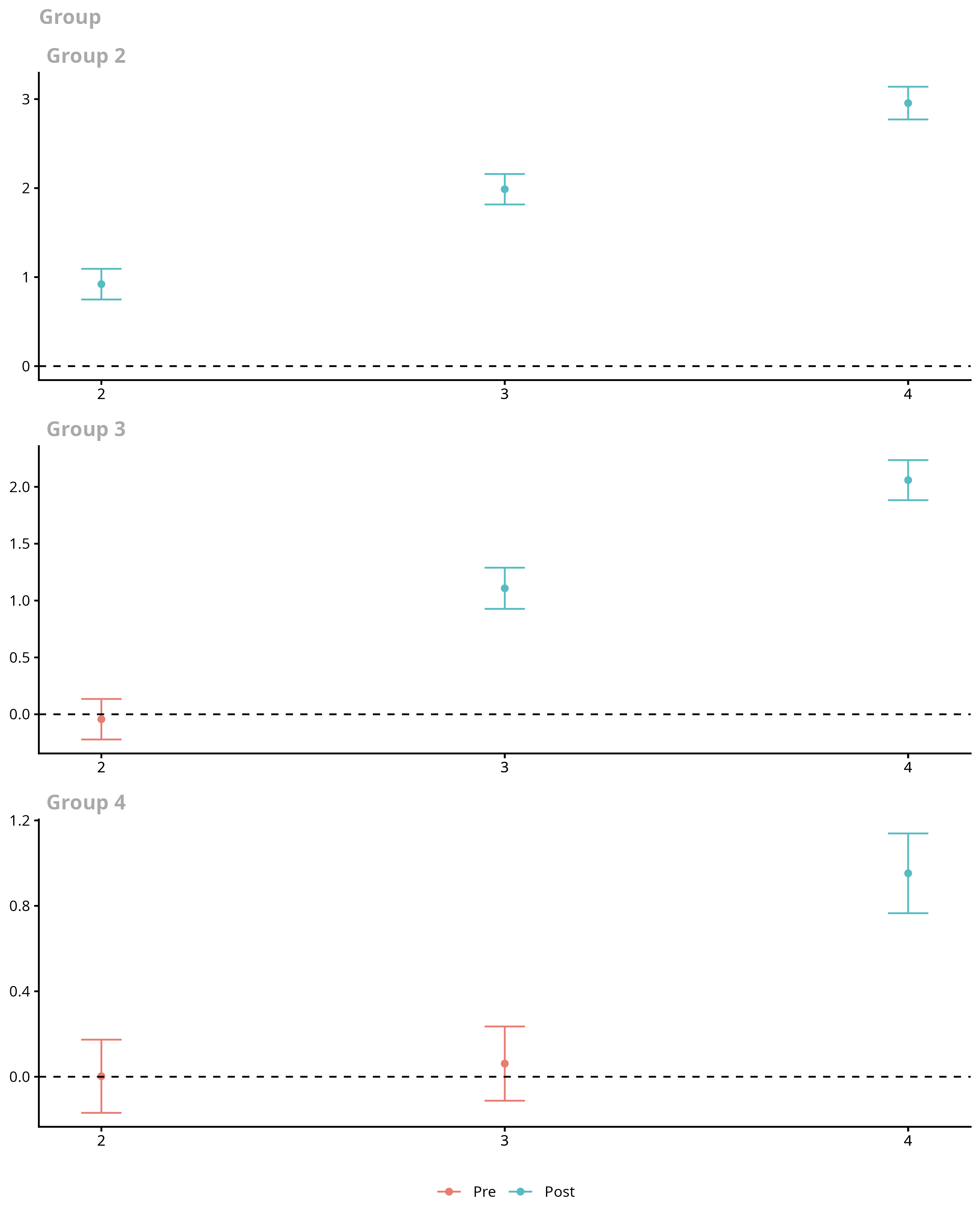
[did] Group-time ATT — att_gt()
The core estimate — where the causal quantity itself is computed.
Estimate ATT(g,t) for every cohort and period against not-yet-treated controls.
Group-time ATT — att_gt() — Difference-in-differences with multiple periods and staggered adoption: ATT(g,t) with clean (not-yet-treated) controls.
att <- att_gt("Y", "period", "id", "first.treat", data = panel)
- No comments on this step yet — be the first.
Log in to comment on this step.
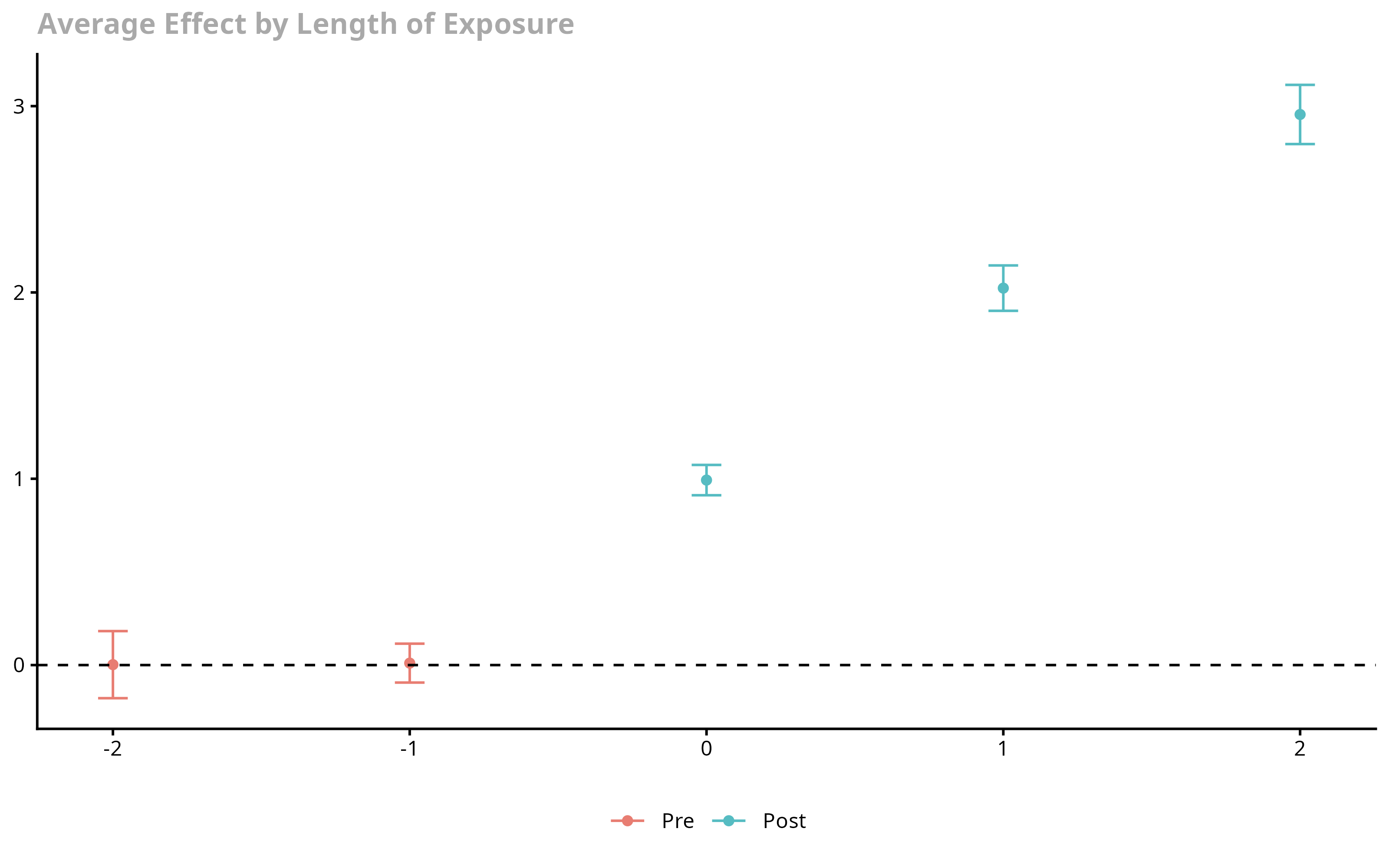
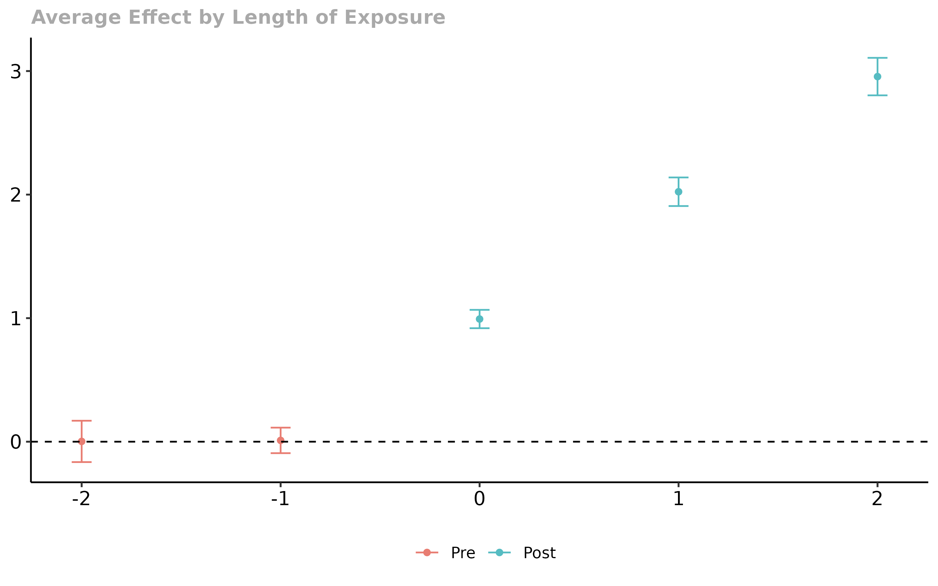
aggte(type = 'dynamic')
Uncertainty quantification — standard errors, intervals, and aggregation.
Aggregate to an event study — effect by length of exposure; pre-periods test parallel trends.
es <- aggte(att, type = "dynamic")
- No comments on this step yet — be the first.
Log in to comment on this step.
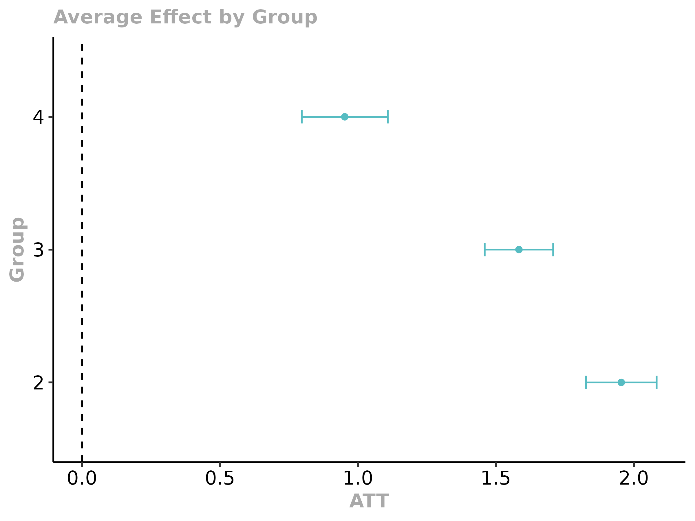
aggte(type = 'group')
Heterogeneity — who is affected, and by how much, not just on average.
Average effect within each treatment cohort.
aggte(att, type = "group")
- No comments on this step yet — be the first.
Log in to comment on this step.
ggdid() event-study plot
Reporting — turn the numbers into a figure or table a reader can act on.
Plot pre-trends + dynamic effects with simultaneous confidence bands.
ggdid(es)
- No comments on this step yet — be the first.
Log in to comment on this step.
Output · what you get 4 figures
Figures reproduced from did — Callaway & Sant'Anna — unofficial community showcase; all credit to the original authors.
The flagship 'did' vignette (Callaway & Sant'Anna). Estimate ATT(g,t) against not-yet-treated controls, then aggregate to a dynamic event study. Unofficial summary.
Discussion (2)
Log in to join the discussion.
The whole point: never compare a treated unit to an already-treated one. att_gt() bakes that in. TWFE users, please switch.
And the dynamic aggregation gives you the event study for free, with simultaneous bands. Chef's kiss.
The not-yet-treated control group is what makes this robust to heterogeneous timing. Great default.