@misc{grf,
  title        = {grf},
  author       = {Athey and Tibshirani and Wager},
  howpublished = {\url{https://grf-labs.github.io/grf/}},
  note         = {Software / documentation}
}The full GRF HTE playbook: cross-fit nuisances → causal forest → calibration → AIPW ATE → BLP → RATE → policy.
Input · what goes in
A randomized/observational study: covariate matrix X, binary treatment W, outcome Y.
Show data format & exampleHide example
Format — one row per unit. A covariate matrix X (numeric), a binary treatment W ∈ {0,1}, and an outcome Y.
  X1     X2    X3    W    Y
 0.42  -1.1   0     1   3.10
-0.07   0.6   1     0   1.85
 1.20   0.3   0     1   4.02
Pipeline · the recipe ⑂ has parallel branches
↑ Click any step in the diagram to read its logic, code, assumptions & discussion.
[GRF] Regression forest
Data preparation — shapes the raw inputs into what the estimator expects.
Cross-fit Y.hat = E[Y|X] and W.hat = E[W|X] so the causal forest splits on orthogonalized residuals.
Regression forest — Honest non-parametric regression for E[Y|X], with out-of-bag predictions and pointwise CIs.
rf <- regression_forest(X, Y)
Y.hat <- predict(rf)$predictions
- No comments on this step yet — be the first.
Log in to comment on this step.
[GRF] Causal forest
The core estimate — where the causal quantity itself is computed.
Grow the causal forest on the residualized moments; get OOB CATEs.
Causal forest — Honest random forest for heterogeneous treatment effects — CATE for a binary treatment via GRF moment conditions.
cf <- causal_forest(X, Y, W) # Y.hat, W.hat cross-fit
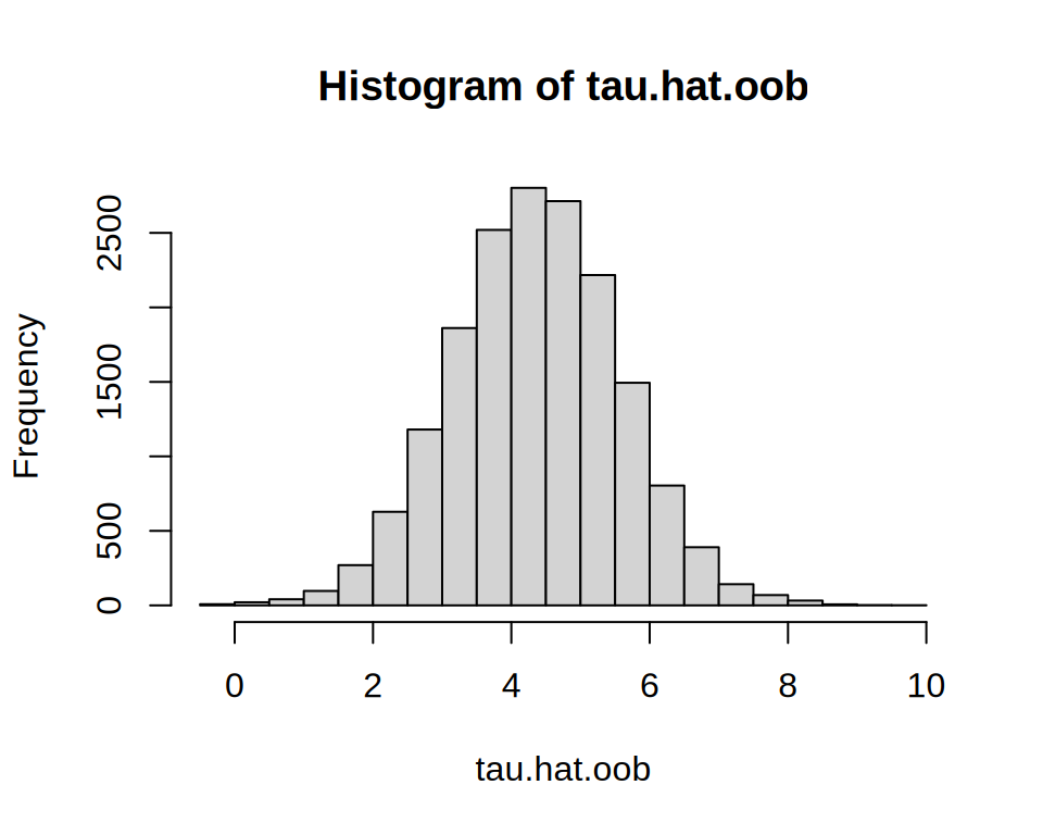
tau.hat <- predict(cf)$predictions # OOB CATEs
- No comments on this step yet — be the first.
Log in to comment on this step.
test_calibration()
A pre-flight check — run this before trusting any estimate downstream.
Regress AIPW scores on mean-forest and differential-forest predictions; the two coefficients should be ≈ 1.
test_calibration(cf) # mean & differential forest coefficients ≈ 1?
- No comments on this step yet — be the first.
Log in to comment on this step.
[GRF] AIPW average treatment effect
Uncertainty quantification — standard errors, intervals, and aggregation.
Doubly-robust ATE (and ATT) as the headline number.
AIPW average treatment effect — Doubly-robust ATE / ATT / ATC / overlap-weighted effect from a trained causal forest, via augmented IPW.
average_treatment_effect(cf, target.sample = "all")      # ATE
average_treatment_effect(cf, target.sample = "treated")  # ATT
- No comments on this step yet — be the first.
Log in to comment on this step.
best_linear_projection()
Heterogeneity — who is affected, and by how much, not just on average.
Project the CATE onto a few interpretable covariates to describe who benefits.
best_linear_projection(cf, X[, c("age", "prior")])
- No comments on this step yet — be the first.
Log in to comment on this step.
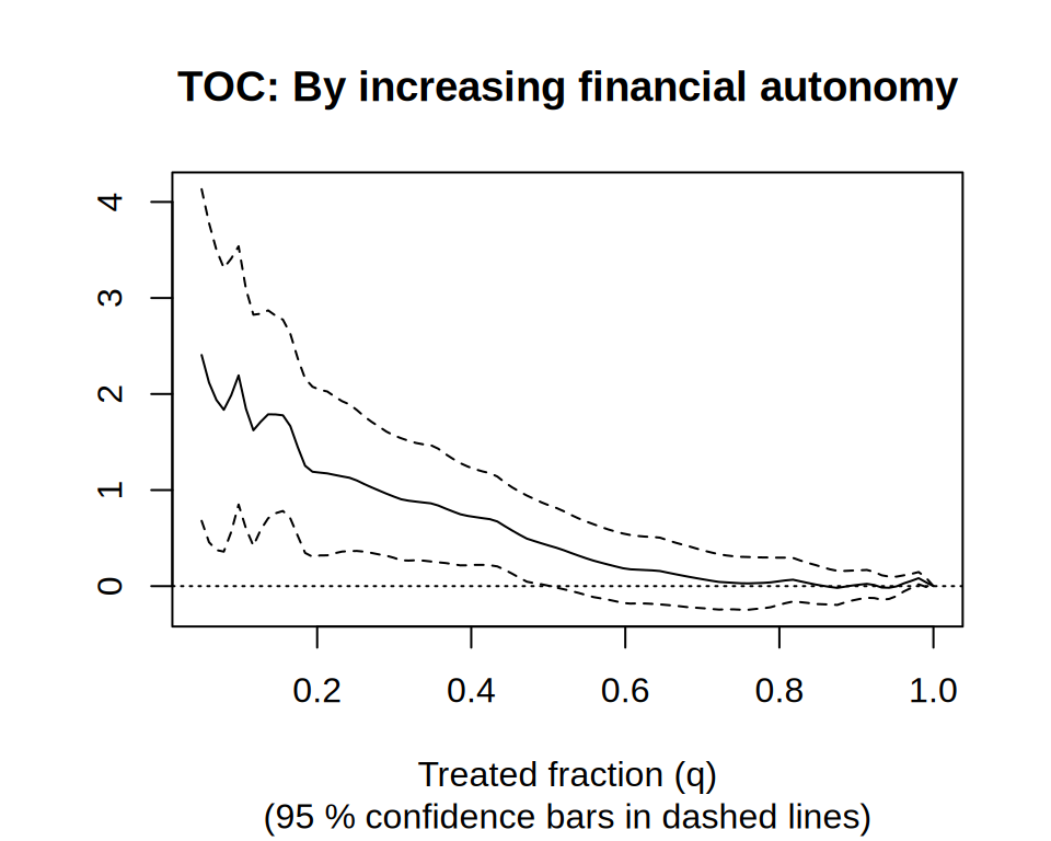
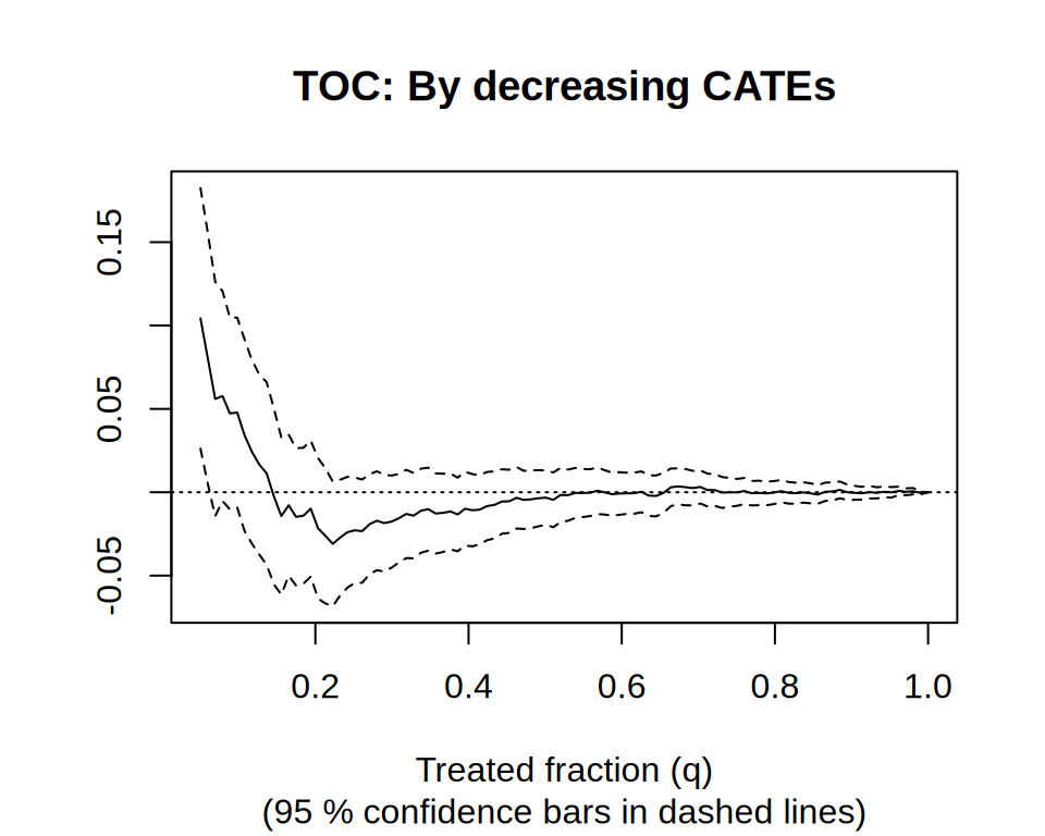
[GRF] Rank-weighted ATE — RATE / AUTOC / Qini
Heterogeneity — who is affected, and by how much, not just on average.
AUTOC on a held-out evaluation forest: is the heterogeneity real and useful for targeting?
Rank-weighted ATE — RATE / AUTOC / Qini — Evaluate how well a CATE estimate prioritizes treatment: TOC curve, AUTOC and Qini with confidence intervals.
rate <- rank_average_treatment_effect(eval.forest, priorities = tau.hat)
plot(rate)                          # TOC curve
rate$estimate / rate$std.err        # AUTOC z-stat
- No comments on this step yet — be the first.
Log in to comment on this step.
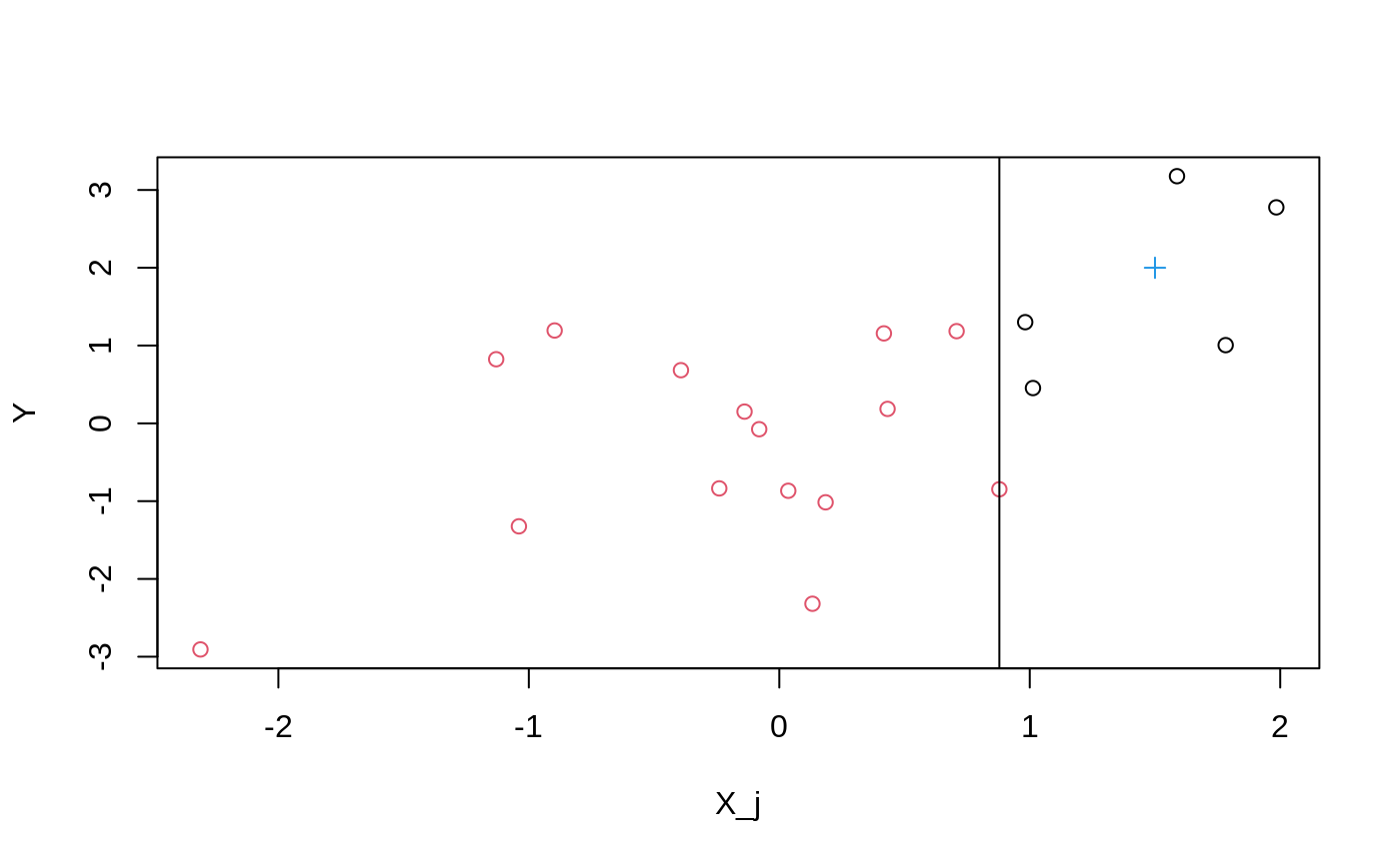
Policy learning (policytree)
A robustness check — does the headline result survive a different lens?
Learn a depth-2 optimal assignment tree from the doubly-robust scores.
library(policytree)
tree <- policy_tree(X, dr.scores, depth = 2)
plot(tree)
- No comments on this step yet — be the first.
Log in to comment on this step.
CATE histogram + targeting report
Reporting — turn the numbers into a figure or table a reader can act on.
Distribution of τ̂(x), BLP table, TOC curve and the learned policy, side by side.
average_treatment_effect(cf, target.weights = w_target)
- No comments on this step yet — be the first.
Log in to comment on this step.
Output · what you get 4 figures
Figures reproduced from grf — Athey, Tibshirani & Wager — unofficial community showcase; all credit to the original authors.
What the GRF docs recommend end-to-end for credible heterogeneous-effect analysis. Nuisances are cross-fit first; the causal forest is then validated (calibration), summarized (AIPW ATE, best linear projection), stress-tested for useful heterogeneity (RATE/AUTOC), and finally turned into a targeting policy. Unofficial summary of the public GRF tutorials.
Discussion (3)
Log in to join the discussion.
This is the canonical order and I wish more papers followed it. Calibration BEFORE you start interpreting subgroups, every time.
And RATE before policy learning — no point optimizing a rule on heterogeneity that isn't there.
Bookmarking this as the onboarding doc for new analysts. The fan-out from the forest into ATE / BLP / RATE / policy is exactly how I teach it.
The fact that one causal_forest object feeds all four downstream branches is the whole pitch for GRF. Compose, don't re-fit.