@misc{grf,
  title        = {grf},
  author       = {Athey and Tibshirani and Wager},
  howpublished = {\url{https://grf-labs.github.io/grf/}},
  note         = {Software / documentation}
}From CATEs to a budgeted treatment policy: causal forest → DR scores → cost matrix → maq Qini curve → pick the budget.
Input · what goes in
CATEs for one or more treatment arms, plus per-unit-per-arm costs.
Show data format & exampleHide example
Format — one row per unit. Covariates X, a treatment factor W with K arms, and outcome Y; optionally a per-arm cost.
  X1    X2   W       Y
 0.4  -1.1  armA   3.1
-0.1   0.6  ctrl   1.8
 1.2   0.3  armB   4.0
Pipeline · the recipe ⑂ has parallel branches
↑ Click any step in the diagram to read its logic, code, assumptions & discussion.
[GRF] Causal forest
The core estimate — where the causal quantity itself is computed.
Fit the forest and produce per-unit CATEs and AIPW scores.
Causal forest — Honest random forest for heterogeneous treatment effects — CATE for a binary treatment via GRF moment conditions.
cf <- causal_forest(X, Y, W)          # Y.hat, W.hat cross-fit
tau.hat <- predict(cf)$predictions    # OOB CATEs
- No comments on this step yet — be the first.
Log in to comment on this step.
Doubly-robust score matrix
Data preparation — shapes the raw inputs into what the estimator expects.
For K arms (or binary), stack the DR scores into the n × K matrix maq consumes.
- No comments on this step yet — be the first.
Log in to comment on this step.
Cost matrix
Data preparation — shapes the raw inputs into what the estimator expects.
Per-unit-per-arm cost (or arm-level cost row); zero-cost arms are allowed as a baseline.
cost <- matrix(unit_cost, n, K) # per-unit, per-arm spend
- No comments on this step yet — be the first.
Log in to comment on this step.
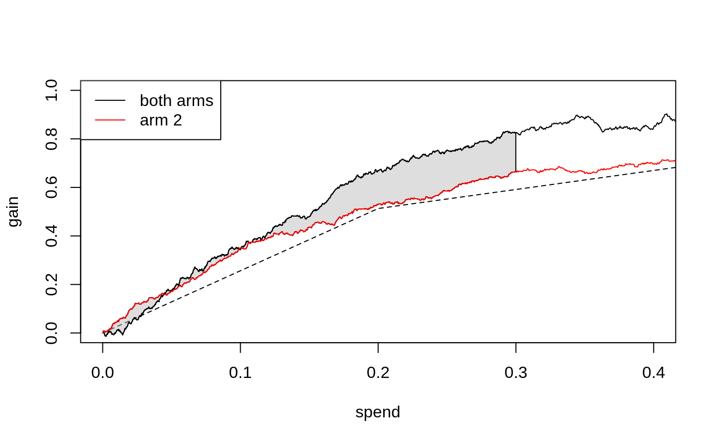
[GRF] Multi-armed Qini curves (maq)
Heterogeneity — who is affected, and by how much, not just on average.
Trace the Pareto frontier of expected gain vs total spend, with bootstrap CIs.
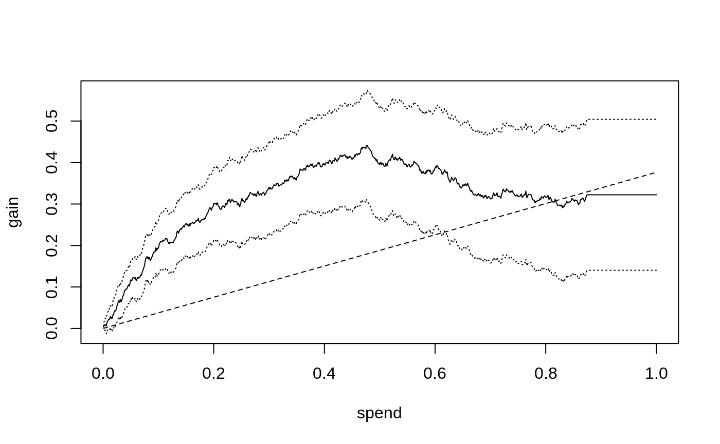
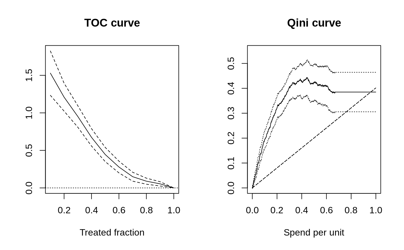
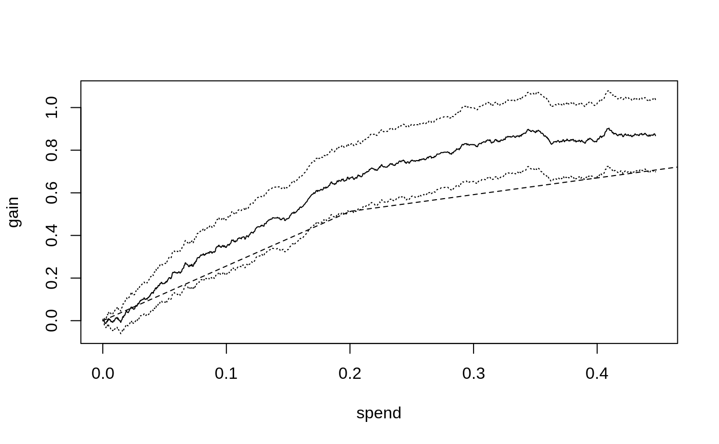
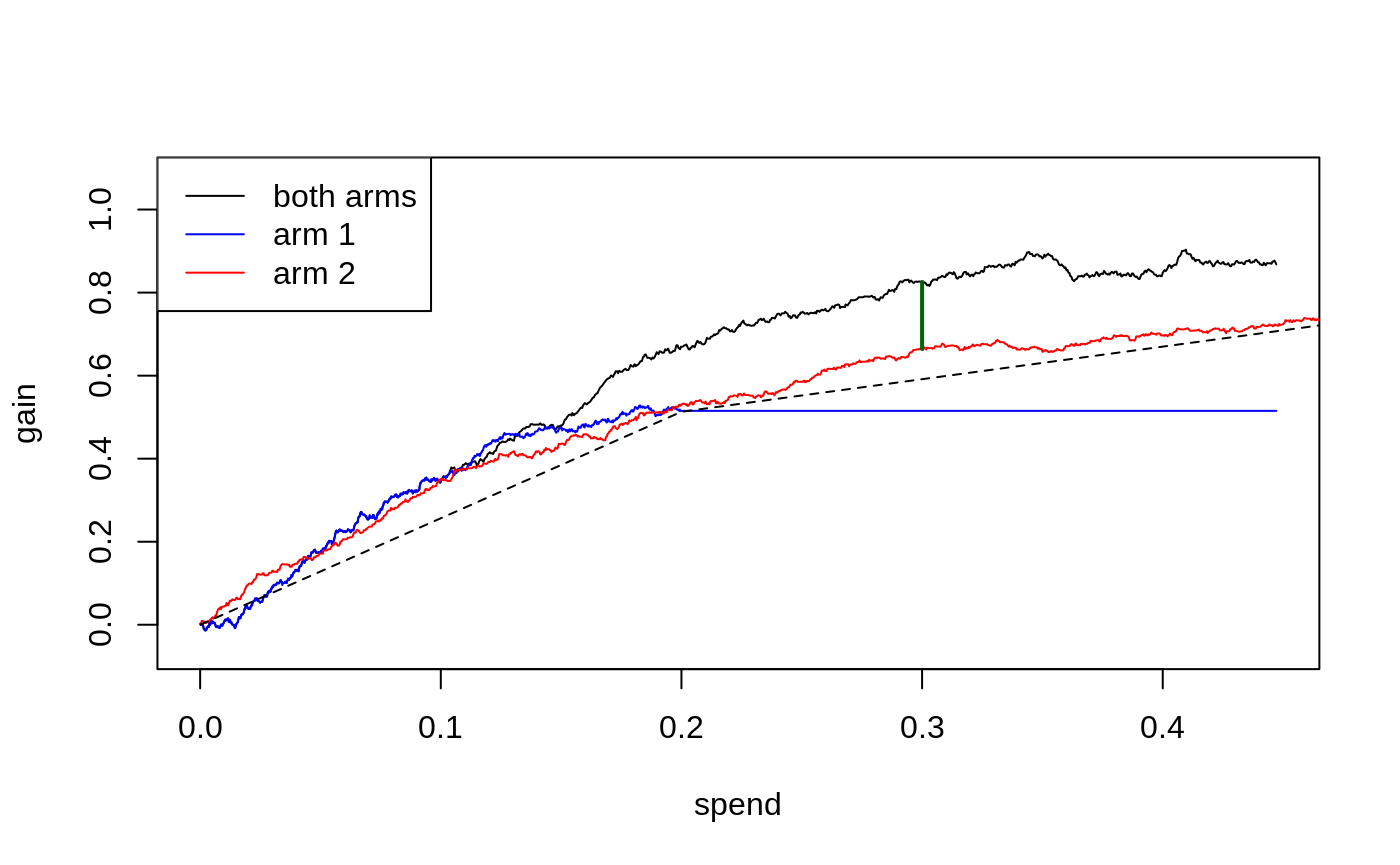
Multi-armed Qini curves (maq) — Cost-aware Qini curves with K treatment arms and per-unit costs — pick the arm and the budget jointly.
library(maq)
mq <- maq(DR.scores, cost, R = 200)
plot(mq); average_gain(mq, spend = 0.3)
- No comments on this step yet — be the first.
Log in to comment on this step.
Pick the budget; report the gain
Reporting — turn the numbers into a figure or table a reader can act on.
Read off the spend that hits a planned ROI; report average_gain() with a CI at that operating point.
- No comments on this step yet — be the first.
Log in to comment on this step.
Output · what you get 5 figures
Figures reproduced from grf — Athey, Tibshirani & Wager — unofficial community showcase; all credit to the original authors.
The GRF 'Qini curves' tutorial. Targeting in the real world has a budget and per-unit costs; the maq sister package turns CATEs into a Pareto frontier of expected-gain vs spend so you can pick the operating point honestly. Unofficial summary.
Discussion (0)
Log in to join the discussion.