@misc{fixest,
  title        = {fixest},
  author       = {Laurent Bergé},
  howpublished = {\url{https://lrberge.github.io/fixest/}},
  note         = {Software / documentation}
}Fast fixed-effects event study that survives staggered timing — sunab() vs naive TWFE, plotted against the truth.
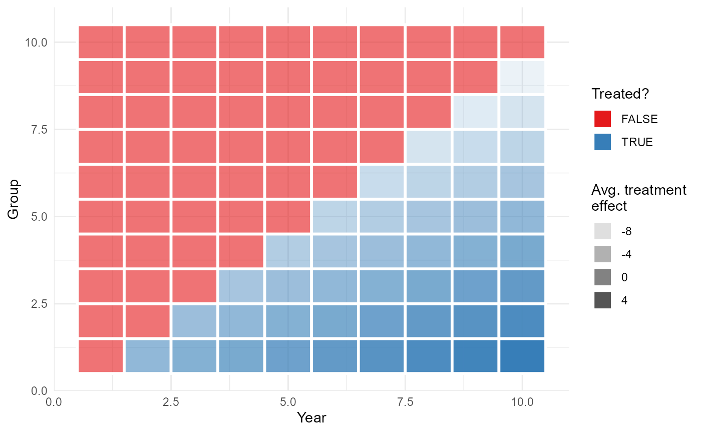
Input · what goes in
A panel with staggered treatment cohorts: unit id, period, cohort (first-treatment period), and an outcome.
Show data format & exampleHide example
Format — one row per (unit, period). cohort = first treated period.
 id  period  cohort   y
  1      1       3    2.0
  1      2       3    2.1
  2      1       5    1.8
Pipeline · the recipe ⑂ has parallel branches
↑ Click any step in the diagram to read its logic, code, assumptions & discussion.
Assemble panel with cohort timing
Data preparation — shapes the raw inputs into what the estimator expects.
Panel id × period; cohort = the period each unit is first treated.
data(base_stagg)
- No comments on this step yet — be the first.
Log in to comment on this step.
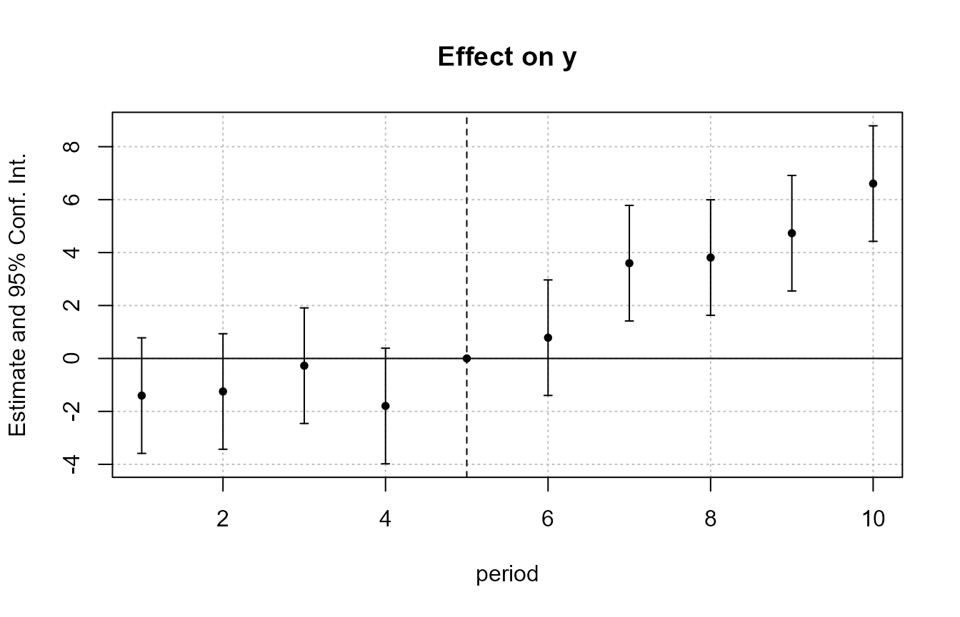
[fixest] Sun & Abraham event study — sunab()
The core estimate — where the causal quantity itself is computed.
Fit feols with sunab(cohort, period) — interaction-weighted, robust to heterogeneous timing.
Sun & Abraham event study — sunab() — Interaction-weighted event-study estimator robust to heterogeneous treatment timing, in a fast fixed-effects framework.
m <- feols(y ~ sunab(year_treated, year) | id + year, base_stagg)
- No comments on this step yet — be the first.
Log in to comment on this step.
Naive TWFE comparison
A robustness check — does the headline result survive a different lens?
Estimate plain TWFE event-study to see the bias Sun-Abraham corrects.
twfe <- feols(y ~ i(time_to_treat, ref = -1) | id + year, base_stagg)
- No comments on this step yet — be the first.
Log in to comment on this step.
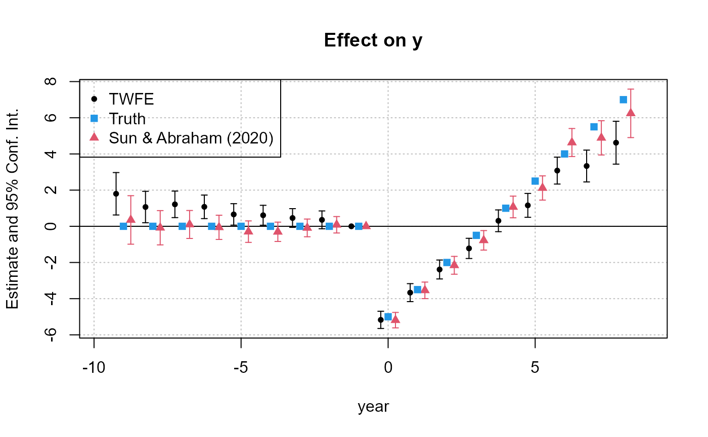
iplot(): SA20 vs TWFE vs truth
Reporting — turn the numbers into a figure or table a reader can act on.
Overlay the event-study coefficients; Sun-Abraham tracks the true effect, TWFE drifts.
iplot(list(m, twfe))
- No comments on this step yet — be the first.
Log in to comment on this step.
Output · what you get 3 figures
Figures reproduced from fixest — Laurent Bergé — unofficial community showcase; all credit to the original authors.
From the fixest walkthrough. Build a staggered panel, fit the Sun-Abraham interaction-weighted event study, and compare it to naive TWFE. Unofficial summary.
Discussion (2)
Log in to join the discussion.
feols is stupid fast and sunab() makes the SA correction a one-liner. No reason to hand-roll event studies anymore.
Nice complement to the did package — same idea (don't trust naive TWFE under staggered timing), FE flavour.
Exactly. iplot() overlaying SA20 vs TWFE vs truth is the clearest illustration of the bias I've seen.