@misc{adjustedcurves,
  title        = {adjustedCurves},
  author       = {Robin Denz},
  howpublished = {\url{https://robindenz1.github.io/adjustedCurves/}},
  note         = {Software / documentation}
}Replace the raw Kaplan-Meier comparison with curves de-confounded by IPTW or the g-formula, with bootstrap bands. Collapse to interpretable summaries — RMST difference up to τ, or survival probability at a clinical horizon — instead of a hazard ratio nobody reads.
Input · what goes in
Right-censored time-to-event data: an event time, an event/censoring indicator, a treatment, and the confounders.
Show data format & exampleHide example
Format — one row per unit: time, status (1=event, 0=censored), group (treatment), confounders x*.
library(adjustedCurves)
adj <- adjustedsurv(data=df, variable='group', ev_time='time',
                    event='status', method='iptw_km',
                    treatment_model=glm(group ~ x1 + x2, family='binomial'))
plot(adj)
Pipeline · the recipe ⑂ has parallel branches
↑ Click any step in the diagram to read its logic, code, assumptions & discussion.
Time-to-event, treatment, confounders
Data preparation — shapes the raw inputs into what the estimator expects.
Set up the censored outcome, the treatment, and the confounders of treatment assignment.
# time (T), status (event 1/0), group (treatment), x1,x2 (confounders)
- No comments on this step yet — be the first.
Log in to comment on this step.
Adjust for confounding (IPTW / g-formula)
The core estimate — where the causal quantity itself is computed.
Weight by the inverse propensity of treatment (or standardise via an outcome model) and form a weighted survival estimate.
adjustedsurv(data=df, variable='group', ev_time='time',
             event='status', method='iptw_km', treatment_model=ps)
- No comments on this step yet — be the first.
Log in to comment on this step.
Curves with confidence bands
Uncertainty quantification — standard errors, intervals, and aggregation.
Bootstrap or asymptotic variance gives pointwise (and simultaneous) bands around each adjusted curve.
adjustedsurv(..., conf_int=TRUE, bootstrap=TRUE)
- No comments on this step yet — be the first.
Log in to comment on this step.
Summaries: RMST difference, survival at t
Reporting — turn the numbers into a figure or table a reader can act on.
Collapse the curves to interpretable numbers: restricted mean survival time, or survival probability at a chosen horizon.
adjusted_rmst(adj, to=5)
- No comments on this step yet — be the first.
Log in to comment on this step.
Output · what you get 2 figures
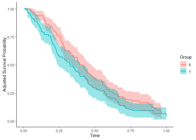
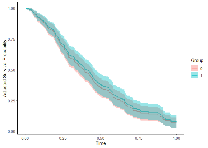
Figures reproduced from adjustedCurves — Robin Denz — unofficial community showcase; all credit to the original authors.
⚠️ Unofficial community showcase of adjustedcurves. Not affiliated with the authors; all credit to them.
Compare survival between treatment groups after removing confounding — via IPTW, the g-formula or AIPW — instead of a raw Kaplan-Meier that quietly bakes in selection.
Discussion (2)
Log in to join the discussion.
Raw Kaplan-Meier between treatment groups in an observational study is the mistake I see most. IPTW-adjusted curves should be the default.
Reporting the RMST difference alongside the curves is the part clinicians actually act on. Good to see it as its own step.
Yes — survival-at-t plus RMST difference communicates far better than a hazard ratio nobody can interpret.