Workflow·5 steps·branched

Smooth signals with a local linear forest

@grf ✓ P D · Jun 2, 2026 · 807 views

@misc{grf,
  title        = {grf},
  author       = {Athey and Tibshirani and Wager},
  howpublished = {\url{https://grf-labs.github.io/grf/}},
  note         = {Software / documentation}
}

Summary by StatsDoge

When the conditional mean is smooth: regression forest baseline → ll_regression_forest → tuning → diagnostics.

Input · what goes in

Outcome Y with a smooth dependence on continuous covariates X.

Show data format & exampleHide example

Format — one row per unit. A covariate matrix X and an outcome Y (no treatment needed).

  X1     X2    X3     Y
 0.42  -1.1   0.2   3.10
-0.07   0.6  -0.5   1.85
 1.20   0.3   0.1   4.02

Pipeline · the recipe ⑂ has parallel branches

↑ Click any step in the diagram to read its logic, code, assumptions & discussion.

Estimation

[GRF] Regression forest

The core estimate — where the causal quantity itself is computed.

What happens here

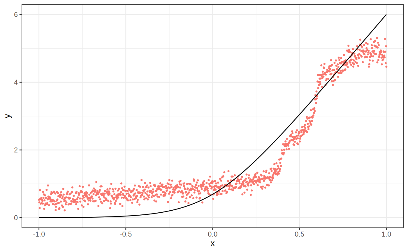
Baseline E[Y|X] fit — establish the score to beat.

Formula

\hat\mu(x)=\mathbb{E}\!\left[\,Y\mid X=x\, ight]

The estimator

Regression forest — Honest non-parametric regression for E[Y|X], with out-of-bag predictions and pointwise CIs.

OTHER Code @ v2.6.1 ↗ Paper ↗

Reads from the input data Feeds into #5

Key code

rf <- regression_forest(X, Y)
Y.hat <- predict(rf)$predictions

Discussion on this step (0)

No comments on this step yet — be the first.

Estimation

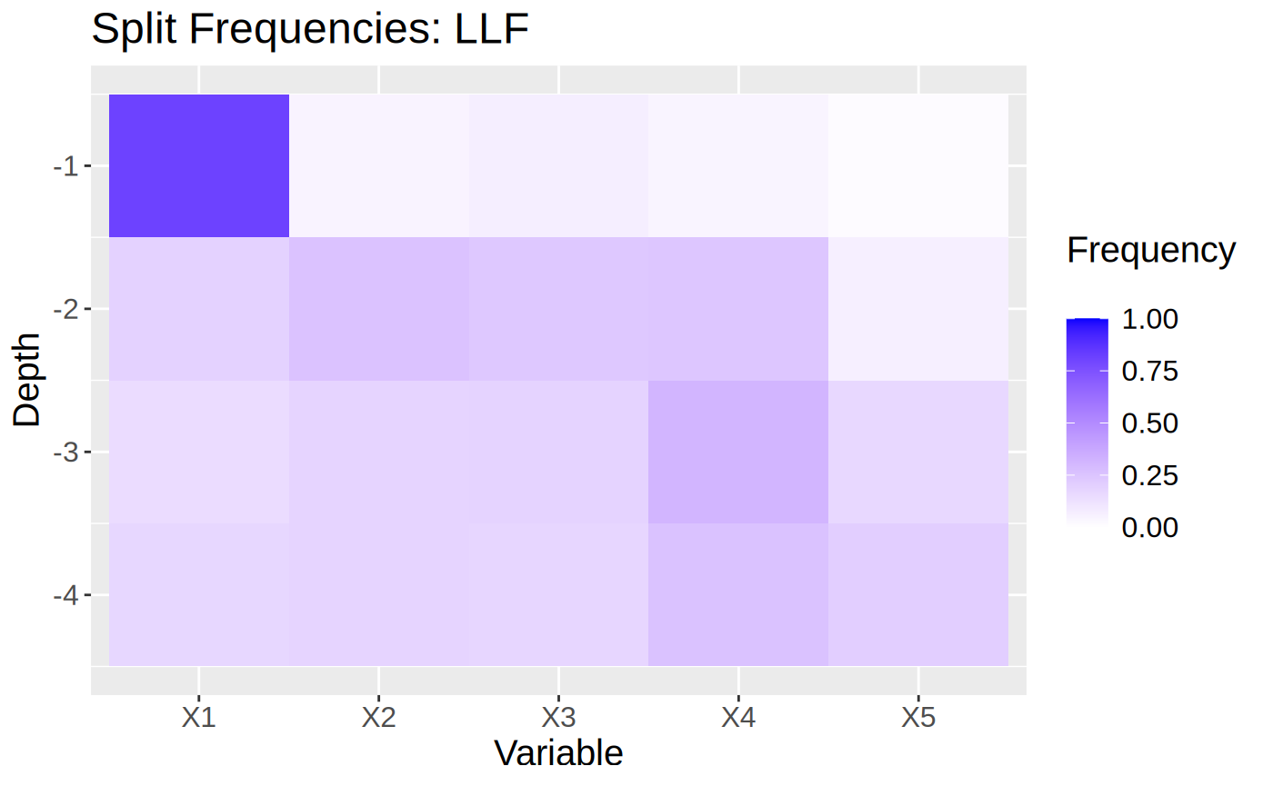
[GRF] Local linear forest

The core estimate — where the causal quantity itself is computed.

What happens here

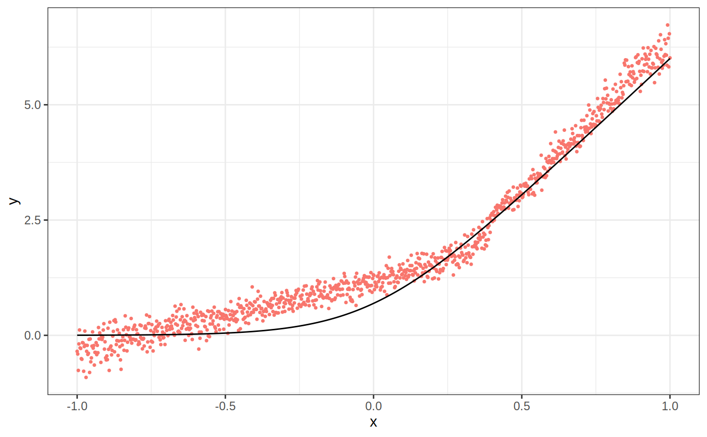
Fit with a chosen set of `linear.correction.variables` (typically the smoothest covariates).

Formula

\hat\mu(x)\approx\hat\mu(x_0)+(x-x_0)^ op\hat heta(x_0)

The estimator

Local linear forest — Random forest with a local linear correction — smoother fits and better extrapolation for smooth signals.

OTHER Code @ v2.6.1 ↗ Paper ↗

Reads from the input data Feeds into #3

Key code

llf <- ll_regression_forest(X, Y)
predict(llf, X.test, linear.correction.variables = 1:ncol(X))

Discussion on this step (0)

No comments on this step yet — be the first.

Diagnostic / pre-tests

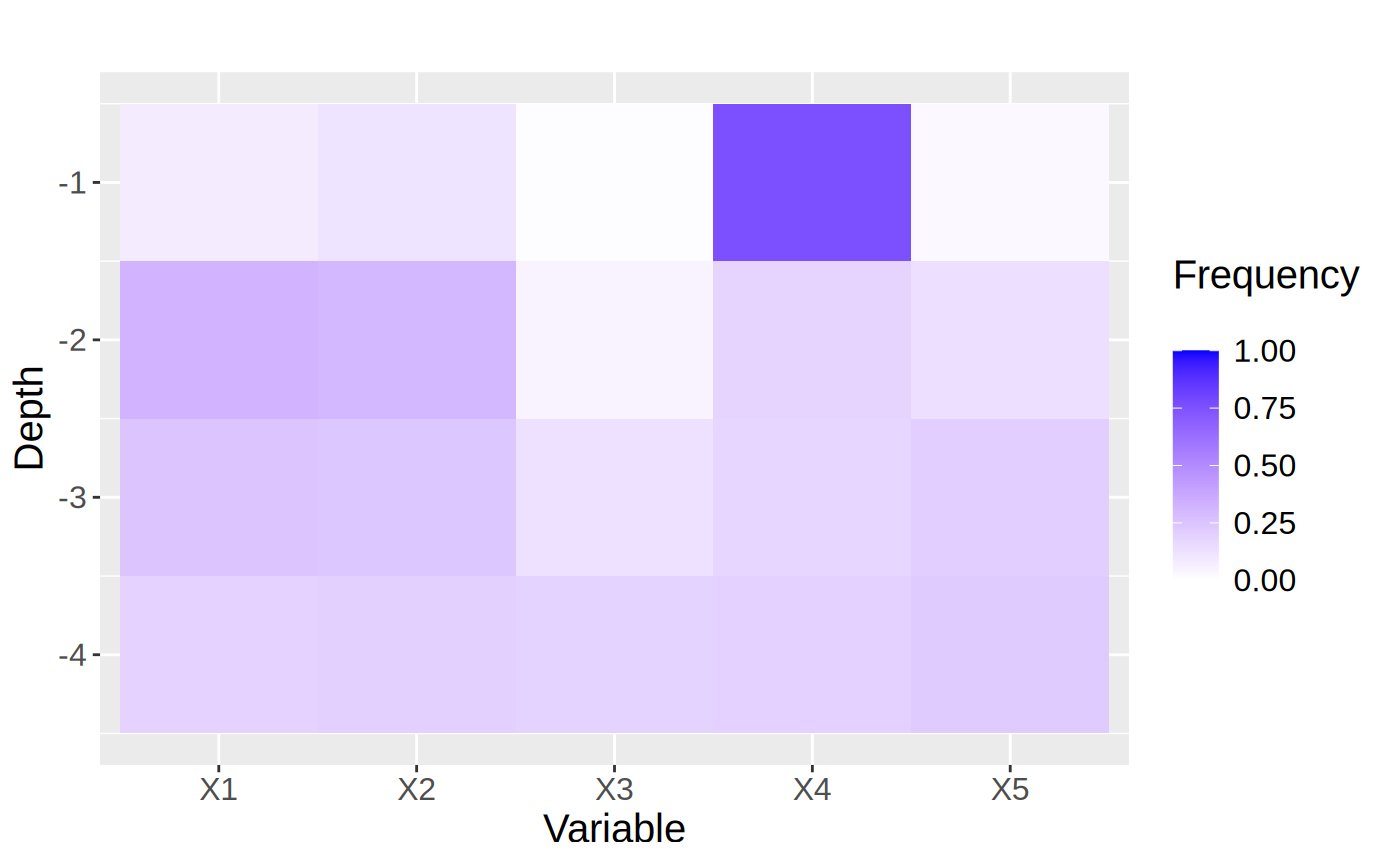
Tune λ via cross-validation

A pre-flight check — run this before trusting any estimate downstream.

What happens here

GRF ships `tune.ll.regression.forest`-style CV; pick the ridge penalty that minimizes held-out MSE.

Reads from #2 Feeds into #4

Discussion on this step (0)

No comments on this step yet — be the first.

Diagnostic / pre-tests

Calibration & boundary plot

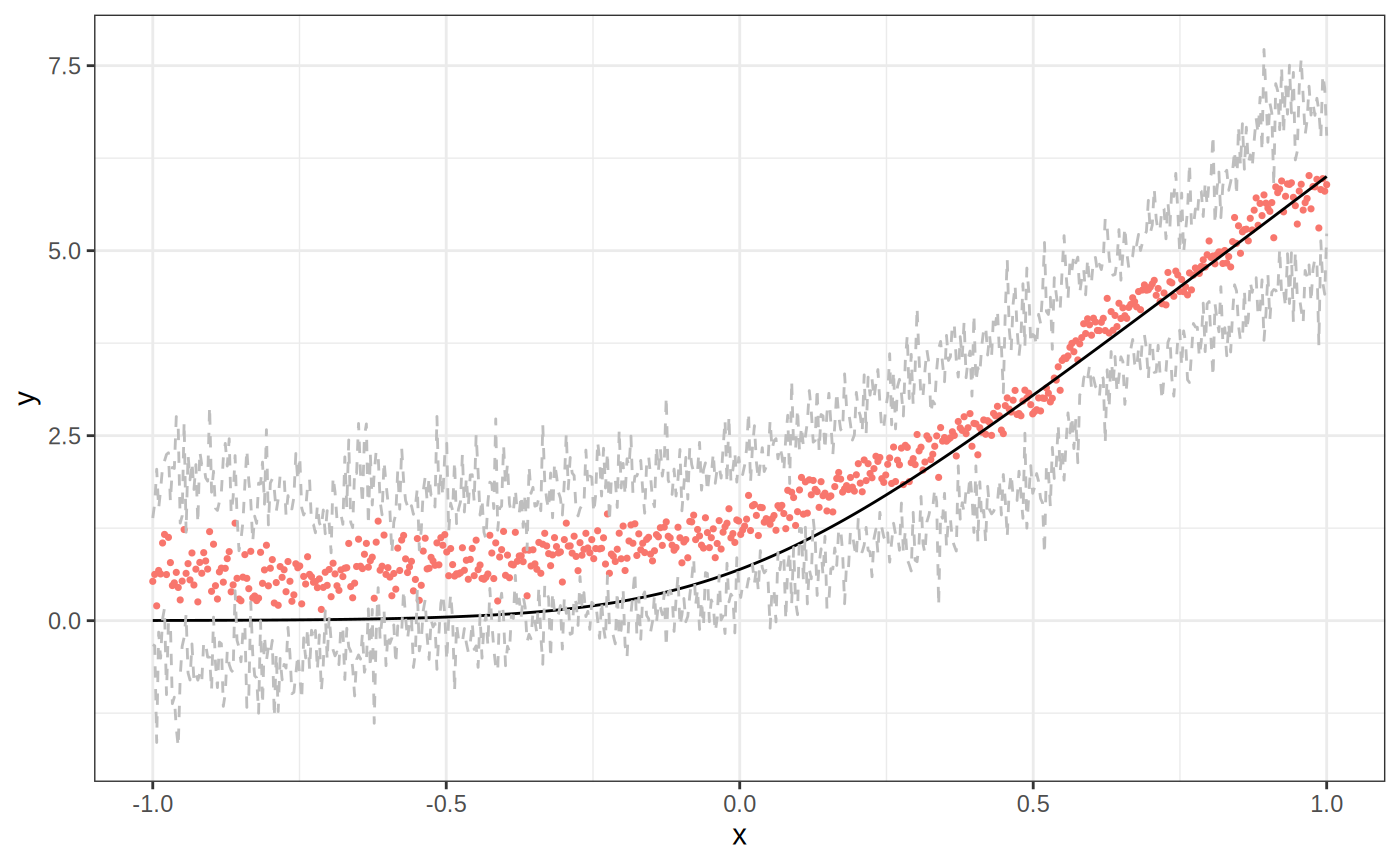
A pre-flight check — run this before trusting any estimate downstream.

What happens here

Predicted vs observed near covariate boundaries — where local linear typically beats plain forests.

Reads from #3 Feeds into #5

Discussion on this step (0)

No comments on this step yet — be the first.

Reporting

Side-by-side comparison

Reporting — turn the numbers into a figure or table a reader can act on.

What happens here

MSE table and overlaid prediction curves; show where llf wins and where it doesn't matter.

Reads from #1#4 Feeds into the final output

Discussion on this step (0)

No comments on this step yet — be the first.

Output · what you get 5 figures

Fig 1A plain regression forest fit vs the smooth truth — note the bias along the trend.

Fig 2The local linear forest tracks the same smooth signal far more closely.

Fig 3Local linear forest fit with 95% confidence bands.

Fig 4Split-frequency heatmap for the regression forest.

Fig 5Split-frequency heatmap for the local linear forest — splits concentrate where the signal bends.

Figures reproduced from grf — Athey, Tibshirani & Wager — unofficial community showcase; all credit to the original authors.

The GRF 'Local linear forests' tutorial. The plain forest can show staircase artifacts near boundaries and on smooth signals; the local linear correction smooths these out and improves extrapolation. Unofficial summary.

Smooth signals with a local linear forest

Input · what goes in

Pipeline · the recipe ⑂ has parallel branches

Output · what you get 5 figures

Discussion (0)