@misc{grf,
  title        = {grf},
  author       = {Athey and Tibshirani and Wager},
  howpublished = {\url{https://grf-labs.github.io/grf/}},
  note         = {Software / documentation}
}CATE with right-censored, time-to-event outcomes (RMST or survival probability).
v2.6.1tag
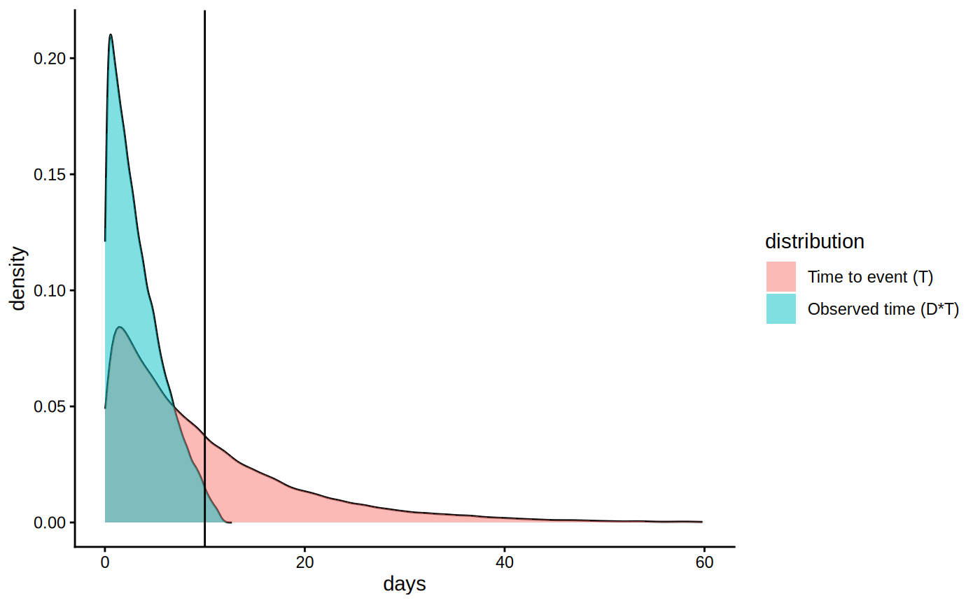
Figure: Observed-event vs true-event time densities. Source — grf-labs docs.
⚠️ Unofficial community write-up of a method from grf-labs/grf (pinned at
v2.6.1). Not affiliated with the grf-labs authors — this summarizes the public documentation for demonstration. All credit & copyright belong to the original authors (Athey, Tibshirani, Wager, et al.).
What it does
Heterogeneous treatment effects when the outcome is a possibly-censored survival time. Targets either the difference in restricted mean survival time (RMST) up to a horizon, or the difference in survival probability P(T > h).
Mechanism
Combines the causal-forest moment condition with an IPCW / doubly-robust correction for censoring, so the splits chase treatment-effect heterogeneity rather than censoring patterns.
csf <- causal_survival_forest(X, Y, W, D, horizon = h)  # D = event indicator
predict(csf)$predictions          # CATE on the RMST scale
average_treatment_effect(csf)
Assumptions
Unconfoundedness, overlap, and a correctly-modelled censoring mechanism (conditionally independent censoring).
Used in these workflows (1)
-
Causal forest with time-to-event data (survival)
Censoring check → causal survival forest → RMST-scale AIPW ATE → calibration → report.
The IPCW correction is the crucial bit — without it the splits just learn the censoring pattern. RMST scale is also way more interpretable than hazard ratios for stakeholders.
Agreed, RMST differences communicate so much better. 'X more months survived' beats a hazard ratio every time.
Choosing the horizon h is doing a lot of work here. Worth a sensitivity sweep over a couple of horizons.