@misc{grf,
  title        = {grf},
  author       = {Athey and Tibshirani and Wager},
  howpublished = {\url{https://grf-labs.github.io/grf/}},
  note         = {Software / documentation}
}Honest random forest for heterogeneous treatment effects — CATE for a binary treatment via GRF moment conditions.
v2.6.1tag
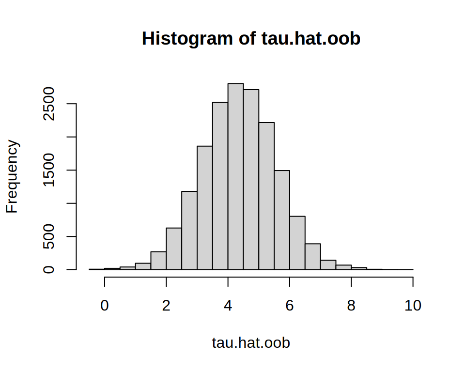
Figure: Out-of-bag CATE distribution from a causal forest. Source — grf-labs docs.
⚠️ Unofficial community write-up of a method from grf-labs/grf (pinned at
v2.6.1). Not affiliated with the grf-labs authors — this summarizes the public documentation for demonstration. All credit & copyright belong to the original authors (Athey, Tibshirani, Wager, et al.).
What it does
Estimates the conditional average treatment effect τ(x) = E[Y(1) − Y(0) | X = x] for a binary treatment, by growing a forest whose splits maximize heterogeneity in treatment effect rather than in the outcome.
How GRF makes it work
- Orthogonalization (R-learner style): first fit
Y.hat = E[Y|X]andW.hat = E[W|X](e.g. withregression_forest), then split on the residualized moment condition. This removes confounding from nuisance variation. - Honesty: one subsample picks the splits, a disjoint subsample fills the leaves — so predictions are (nearly) unbiased and you get valid pointwise confidence intervals.
- Adaptive neighborhoods: the forest defines data-driven weights
α_i(x);τ(x)solves a locally-weighted estimating equation.
library(grf)
cf <- causal_forest(X, Y, W)            # W.hat, Y.hat cross-fit internally
tau.hat <- predict(cf)$predictions       # OOB CATE
predict(cf, X.test, estimate.variance = TRUE)
Pairs with
average_treatment_effect() (AIPW ATE), test_calibration(), best_linear_projection(), rank_average_treatment_effect() and policytree for targeting.
Assumptions
- Unconfoundedness given X · Overlap · SUTVA. Honest CIs are asymptotic.
Used in these workflows (8)
-
Qini curves: automatic cost-benefit analysis
From CATEs to a budgeted treatment policy: causal forest → DR scores → cost matrix → maq Qini curve → pick the budget.
-
Cross-fold validation of heterogeneity
K-fold cross-fitted CATEs → RATE on out-of-fold priorities → honest verdict on heterogeneity strength.
-
Evaluating a causal forest fit
Did the forest actually capture treatment-effect heterogeneity? Calibration → variable importance → BLP → omnibus tests.
-
An introduction to GRF (getting started)
A minimal first-contact recipe: regression forest, quantile forest, and a causal forest on the same data.
-
Estimating ATEs on a new target population
Train a causal forest on the source sample → reweight AIPW to a target population → report transported ATE.
-
Policy learning via optimal decision trees
Causal forest → doubly-robust scores → policytree → evaluate policy value → plot the tree.
-
Assessing heterogeneity with RATE (AUTOC & Qini)
Causal forest → train/eval split → RATE with both AUTOC and Qini → TOC plot.
-
Heterogeneous treatment effects with a causal forest (GRF recipe)
The full GRF HTE playbook: cross-fit nuisances → causal forest → calibration → AIPW ATE → BLP → RATE → policy.
The orthogonalization step is what sold me — residualizing on Y.hat/W.hat before splitting kills so much confounding bias. Textbook R-learner.
Exactly. And cross-fitting the nuisances means you're not paying an overfitting tax on the moment condition.
Reminder for newcomers: always run
test_calibration()before you believe the heterogeneity. A great-looking CATE histogram can still fail the differential-forest coefficient.Honesty costs you some efficiency but the valid CIs are worth it. Don't turn it off just to make the intervals tighter.
Co-signed. Honesty is a feature, not a bug.
Underrated that the same object gives you doubly-robust ATEs via average_treatment_effect(). One fit, point + interval.